Bayesian model averaging (BMA) for uncorrelated relaxed clocks
In previous tutorials, we have described different model selection approaches to select the optimal model (out of a selection of available models) for a data set using marginal likelihood estimation. We have discussed different techniques to estimate the marginal likelihood, by either using path sampling and stepping-stone sampling or using generalized stepping-stone sampling. Although quantifying the marginal likelihood of alternative models is invaluable when it relates to hypothesis testing, model selection and its search for a single best-fit model typically ignores uncertainty about the “correct” model specification and can lead to overconfident inferences (Hoeting et al. 1999). Bayesian model averaging (BMA) approaches have been proposed to explicitly address model uncertainty by forming a posterior distribution over a set of candidate models (Madigan and Raftery 1994). In general, BMA does not provide a method for identifying the most likely model within the candidate set of models, as the aim of BMA is often orthogonal to model selection efforts.
Li and Drummond (2012) have developed a BMA approach in which the candidate set includes a small number of relaxed molecular clock models in Bayesian phylogenetics. Such relaxed clock models present a useful method for removing the assumption of a strict molecular clock. As such, the rate on each branch of the tree is drawn independently and identically from an underlying rate distribution. The two most popular candidates for the rate distribution among branches are the uncorrelated exponential distribution and the uncorrelated lognormal distribution. Apart from these two underlying distributions, BEAUti also offers an underlying gamma distribution to be used for the uncorrelated relaxed clock.
We refer to Lepage et al. (2007) and Baele et al. (2012, 2013) as examples for comparing different clock models to one another.
Setting up Bayesian Model Averaging in BEAUti
After importing a data set, the Clocks panel in BEAUti allows you to specify a molecular clock for your analysis. An overview of the available clock models can be found here.
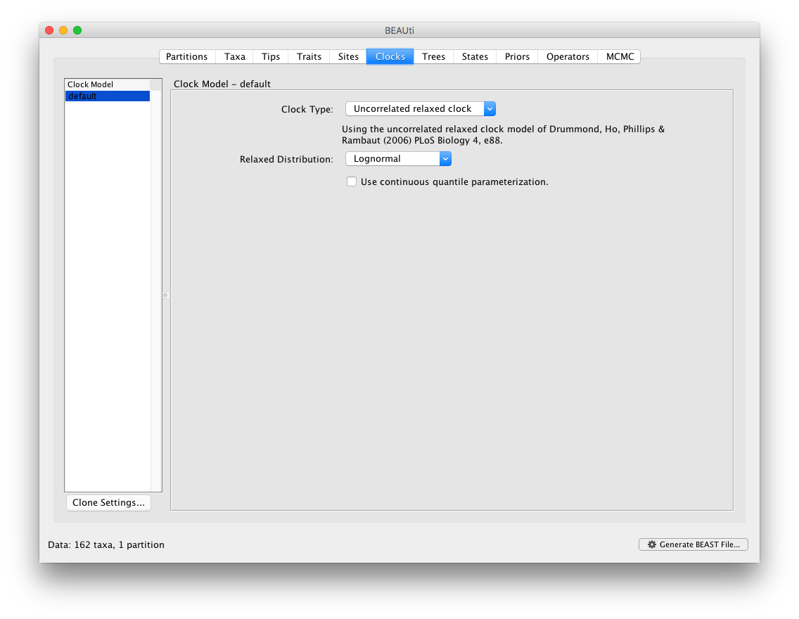
The BMA option is available as part of the “Relaxed Distribution” dropdown menu, after the “Uncorrelated relaxed clock” option has been selected. Note that the BMA approach averages over a selection of uncorrelated relaxed clock models. The strict clock, fixed local clock or random local clock models are hence not part of the mixture of models within BMA.
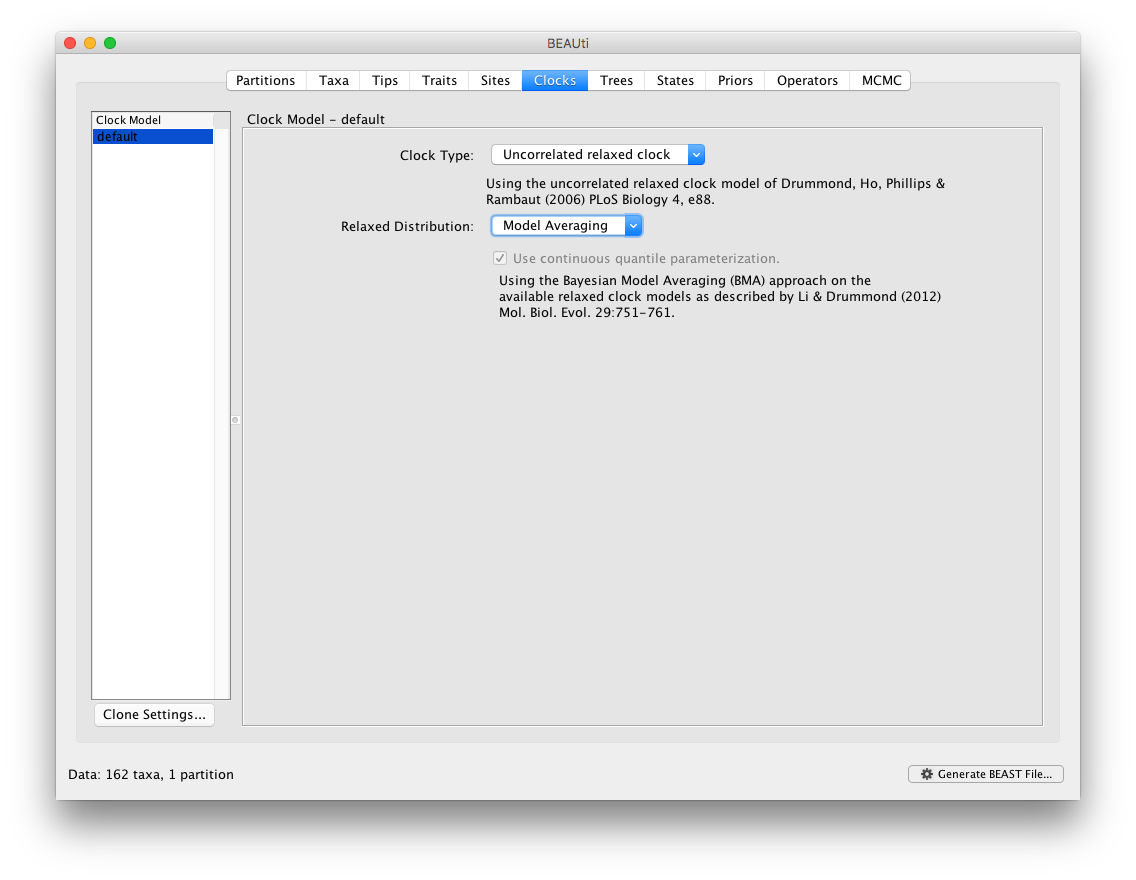
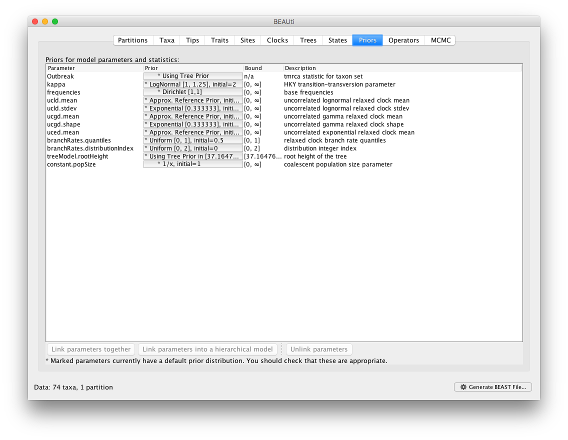
By default, BMA in BEAUti will add all available underlying distributions for the uncorrelated relaxed clock models into the BMA mixture. Specifically, this includes the exponential, lognormal and gamma distributions. In the next section of this tutorial, we show how to extend and/or modify this selection by editing the XML file generated by BEAUti. The following Prior panel then automatically contains suggestions for the prior distributions across all the clock paramaters within the BMA mixture.
Additionally, the corresponding transition kernels for proposing parameter updates and switching between clock models in the BMA mixture are automatically generated in the Operators panel.
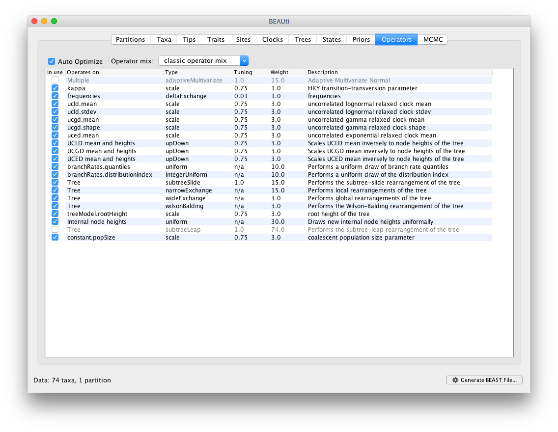
Essentially, selecting the BMA option in the Clocks panel takes care of all the necessary settings within BEAUti. It’s of course possible to edit the prior distributions and the transition kernels at your own convenience.
Modifying Bayesian Model Averaging through XML editing
Using the default mixture of models in BEAUti, the following XML code is generated in the output XML file:
<beast>
    ...
    <mixtureModelBranchRates id="branchRates">
        <treeModel idref="treeModel"/>
        <distribution>
            <logNormalDistributionModel meanInRealSpace="true">
                <mean>
                    <parameter id="ucld.mean" value="1.0"/>
                </mean>
                <stdev>
                    <parameter id="ucld.stdev" value="0.3333333333333333" lower="0.0"/>
                </stdev>
            </logNormalDistributionModel>
        </distribution>
        <distribution>
            <gammaDistributionModel>
                <mean>
                    <parameter id="ucgd.mean" value="1.0"/>
                </mean>
                <shape>
                    <parameter id="ucgd.shape" value="0.3333333333333333" lower="0.0"/>
                </shape>
            </gammaDistributionModel>
        </distribution>
        <distribution>
            <exponentialDistributionModel>
                <mean>
                    <parameter id="uced.mean" value="1.0"/>
                </mean>
            </exponentialDistributionModel>
        </distribution>
        <distributionIndex>
            <parameter id="branchRates.distributionIndex" value="0.0" lower="0.0"/>
        </distributionIndex>
        <rateCategoryQuantiles>
            <parameter id="branchRates.quantiles" value="0.5" lower="0.0" upper="1.0"/>
        </rateCategoryQuantiles>
    </mixtureModelBranchRates>
    ...
</beast>
It’s however quite straight forward to add or replace the provided distributions with underlying distributions of your own choosing. For example, in the BMA paper of Li and Drummond (2012), an inverse Gaussian distribution is used rather than a gamma distribution. In order to create such a mixture of models, the <gammaDistributionModel>…</gammaDistributionModel> block can be replaced by the following XML code:
<inverseGaussianDistributionModel>
    <mean>
        <parameter id="ucid.mean" value="1.0"/>
    </mean>
    <stdev>
        <parameter id="ucid.stdev" value="0.3333333333333333"/>
    </stdev>
</inverseGaussianDistributionModel>
Additionally, the transition kernels for the ucgd.mean and ucgd.shape parameters need to be replaced by the following:
<scaleOperator scaleFactor="0.75" weight="10">
    <parameter idref="ucid.mean"/>
</scaleOperator>
<scaleOperator scaleFactor="0.75" weight="5">
    <parameter idref="ucid.stdev"/>
</scaleOperator>
<upDownOperator scaleFactor="0.75" weight="3">
    <up>
        <parameter idref="ucid.mean"/>
    </up>
    <down>
        <parameter idref="treeModel.allInternalNodeHeights"/>
    </down>
</upDownOperator>
The prior specifications also need to be adjusted, i.e. the priors on ucgd.mean and ucgd.shape need to be removed and the following priors can be added:
<ctmcScalePrior>
    <ctmcScale>
        <parameter idref="ucid.mean"/>
    </ctmcScale>
    <treeModel idref="treeModel"/>
</ctmcScalePrior>
<exponentialPrior mean="0.3333333333333333" offset="0.0">
    <parameter idref="ucid.stdev"/>
</exponentialPrior>
Finally, don’t forget to modify the parameters that are being written to file.
References
J. A. Hoeting, D. Madigan, A. E. Raftery and C. T. Volinsky (1999) Bayesian model averaging: a tutorial. Stat Sci. 14:382-417.
D. Madigan and A. E. Raftery (1994) Model selection and accounting for model uncertainty in graphical models using Occam’s window. J. Am. Stat. Assoc. 89:1535-1546.
W. L. S. Li and A. J. Drummond (2012) Model averaging and Bayes factor calculation of relaxed molecular clocks in Bayesian phylogenetics. Mol. Biol. Evol. 29(2):751-761.
T. Lepage, D. Bryant, H. Philippe and N. Lartillot (2007) A general comparison of relaxed molecular clock models. Mol. Biol. Evol. 24(12):2669-2680.
G. Baele, P. Lemey, T. Bedford, A. Rambaut, M. A. Suchard, M. A. and A. V. Alekseyenko (2012) Improving the accuracy of demographic and molecular clock model comparison while accommodating phylogenetic uncertainty. Mol. Biol. Evol. 29(9), 2157-2167.
G. Baele, W. L. S. Li, A. J. Drummond, M. A. Suchard, and P. Lemey (2013) Accurate model selection of relaxed molecular clocks in Bayesian phylogenetics. Mol. Biol. Evol. 30(2):239-243.