In the first introductory tutorial we looked at importing data into BEAUti, setting up a model and analysis, and running this analysis in BEAST. In this second tutorial, we will analyse the output of that analysis by examining its output file in Tracer and by building a consensus tree and visualising it in FigTree. But first, we explain how to combine the output files of multiple independent replicates (i.e. running the same BEAST XML using different starting seeds). Such a setup can be useful when achieving a good effective sample size for each parameter is computationally cumbersome for example, and multiple hardware resources are available to run independent replicates in parallel.
Combining results from multiple replicates
LogCombiner is distributed as part of the BEAST package and allows you to combine multiple output files into a single output file, which can make for easier post-processing of your analysis. Note that to combine these output files, you’ll have to run LogCombiner twice, once to combine the .log files and once more to combine the .trees files. More information on how to use LogCombiner can be found on its dedicated page. For the remainder of this tutorial, we will assume the presence of a single .log file and a single .trees file.
Inspecting the performance of the transition kernels
A step that’s often forgotten/neglected is to quickly inspect the behavior and/or performance of the various transition kernels (or operators as they’re called in BEAST). At the end of an analysis, a .ops file will typically be created that contains important aspects of the parameter and tree estimation process. For the analysis that we set up during the first tutorial, an apes.ops file is created that will contain content similar to this:
Operator analysis
Operator                                          Tuning   Count      Time     Time/Op  Pr(accept)
scale(kappa)                                      0.289   9642       130      0.01     0.2385
frequencies                                       0.062   9717       155      0.02     0.2409
subtreeSlide(treeModel)                           0.02    289099     2280     0.01     0.2313
Narrow Exchange(treeModel)                                288345     2668     0.01     0.0549
Wide Exchange(treeModel)                                  28842      150      0.01     0.0109
wilsonBalding(treeModel)                                  28874      172      0.01     0.0057
scale(treeModel.rootHeight)                       0.131   28831      242      0.01     0.241
uniform(nodeHeights(treeModel))                           287901     2710     0.01     0.3851
scale(yule.birthRate)                             0.2     28749      103      0.0      0.2399
Typically, the acceptance ratio of a transition kernel will be around 0.234 or higher, depending on the type of operation. Note that it is known to not be the case for certain tree transition kernels, especially so here given the small number of taxa that we’re analysing. The most important thing here is to ascertain that none of the standard transition kernels have an acceptance rate of zero.
Summarizing parameter estimates
Loading the .log files, containing parameter samples from all the parameters in our analysis with exception of the trees and their corresponding branch lengths, into Tracer yields the following screen:
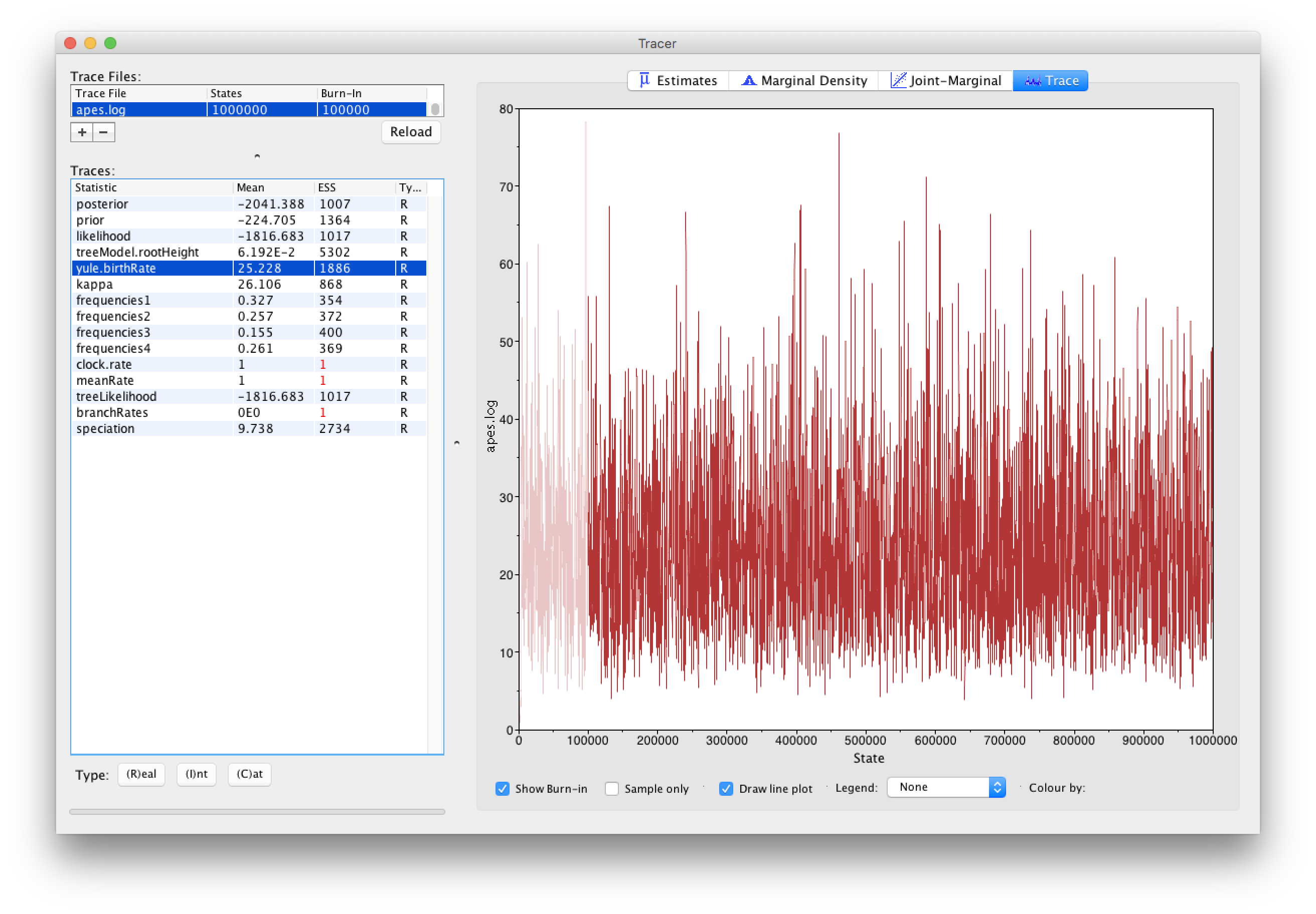
From the Tracer window, it’s clear that the ESS values for all the continuous parameters are more than sufficient to terminate the analysis. Note that ESS values should not be used/estimated for categorical or discrete parameters, and neither for the posterior, likelihood and prior density samples. However, for those latter estimates, low ESS values may reflect underlying problems in estimating certain parameters, so they do have their use for such densities. For discrete parameters, it may be of interest to inspect the traces of those parameters so that proper convergence towards the posterior distribution can be assessed.
Note that constant parameters, i.e. parameters that are not being estimated (such as the clock.rate and the meanRate) or normalizing constants (such as the branchRates), are shown for completeness but need not be inspected for convergence and/or ESS values.
More detailed Tracer tutorials are available, focusing on analysing BEAST output and assessing convergence.
Building an MCC tree
It’s simply not feasible to inspect every tree that was visited during the BEAST analysis, hence we will create a consensus tree summarizing the posterior tree distribution. Within the BEAST package, this is done by constructing a maximum clade credibilty (MCC) tree using the program TreeAnnotator.
Upon running TreeAnnotator, you will be presented with the following window:
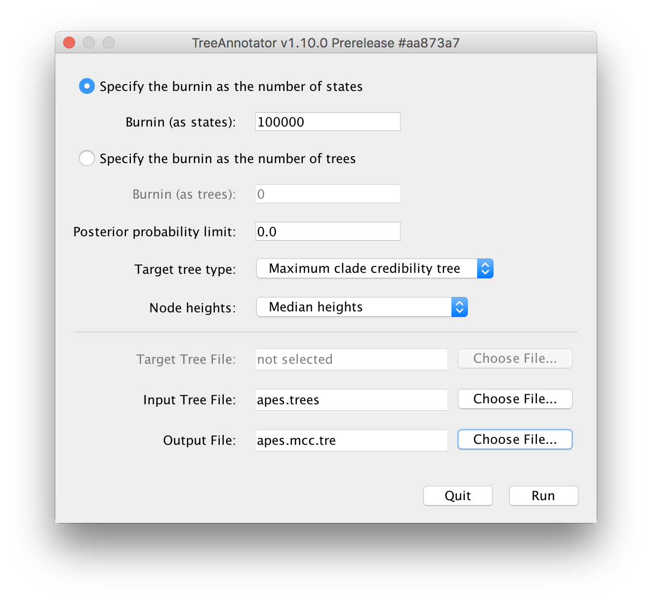
Typically, 10% of the total number of iterations is used as the burn-in for an analysis, provided that this is sufficient to have made it past the actual burn-in phase (which can be inspected/checked in Tracer).
For the Input Tree File, the apes.trees file that generated during the BEAST run needs to be selected.
For the Output File, no such file can be selected but rather it’s file name needs to be entered manually in the following window (where it says `Save As):
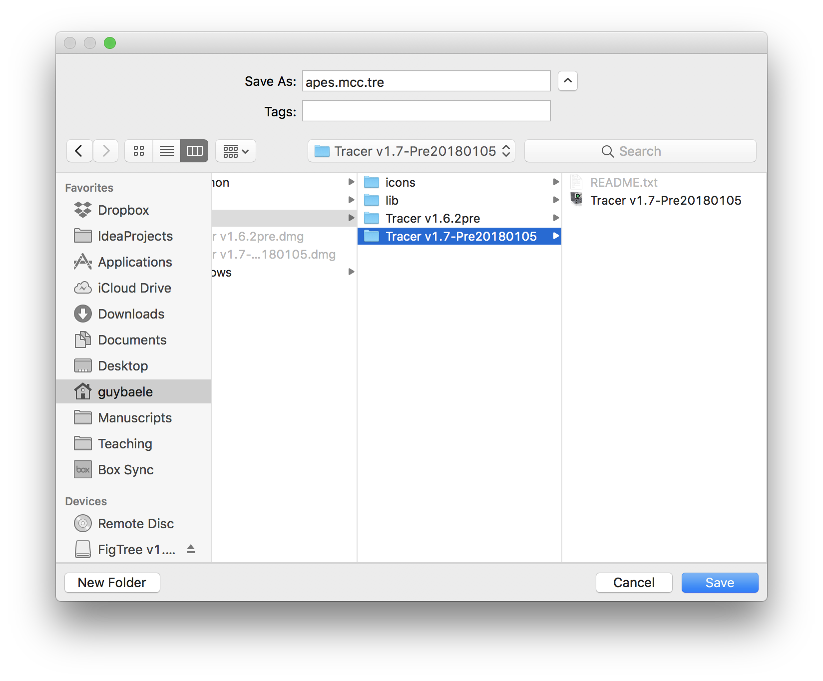
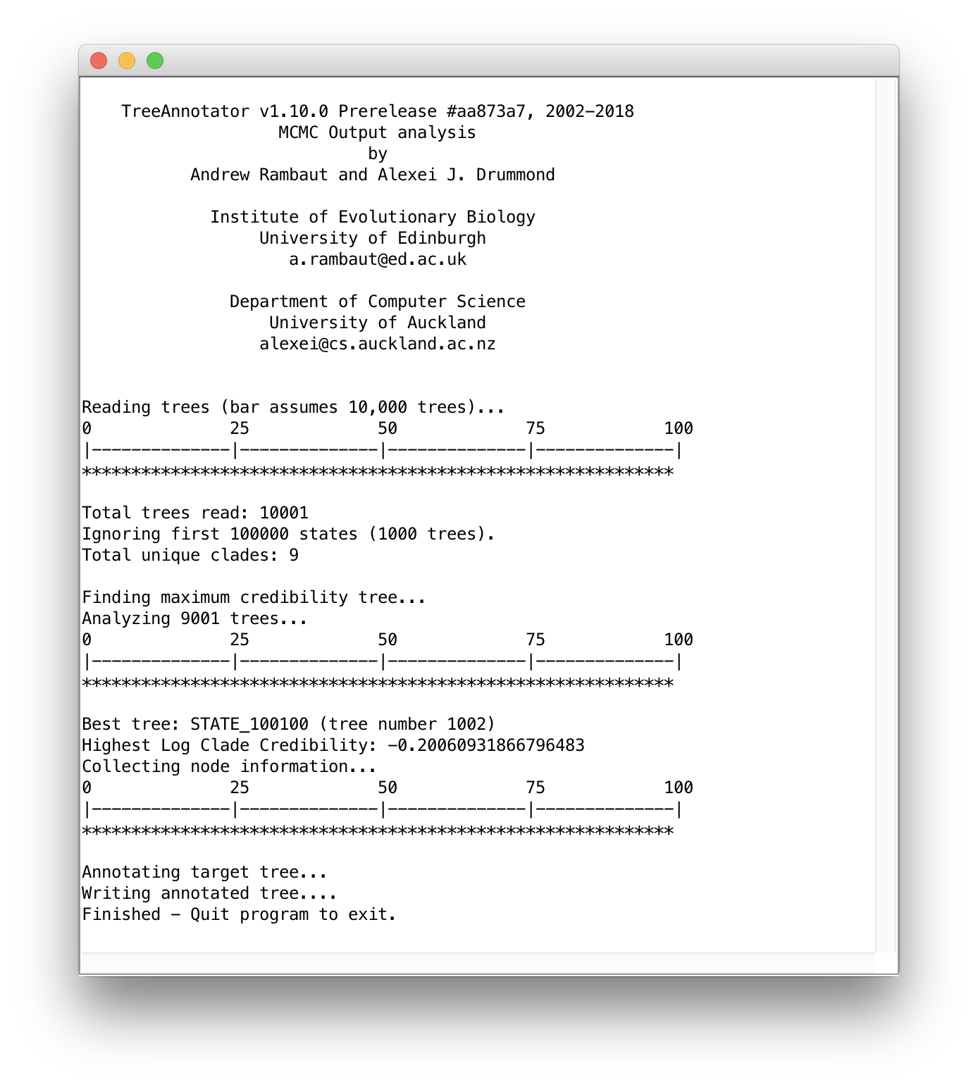
After all the required settings have been entered, you can start constructing the MCC tree by clicking `Run. Progress can monitored in the following window, at the end of which you will be asked to quit the program and the MCC tree will have been written to the selected output file:
Visualising the MCC tree in FigTree
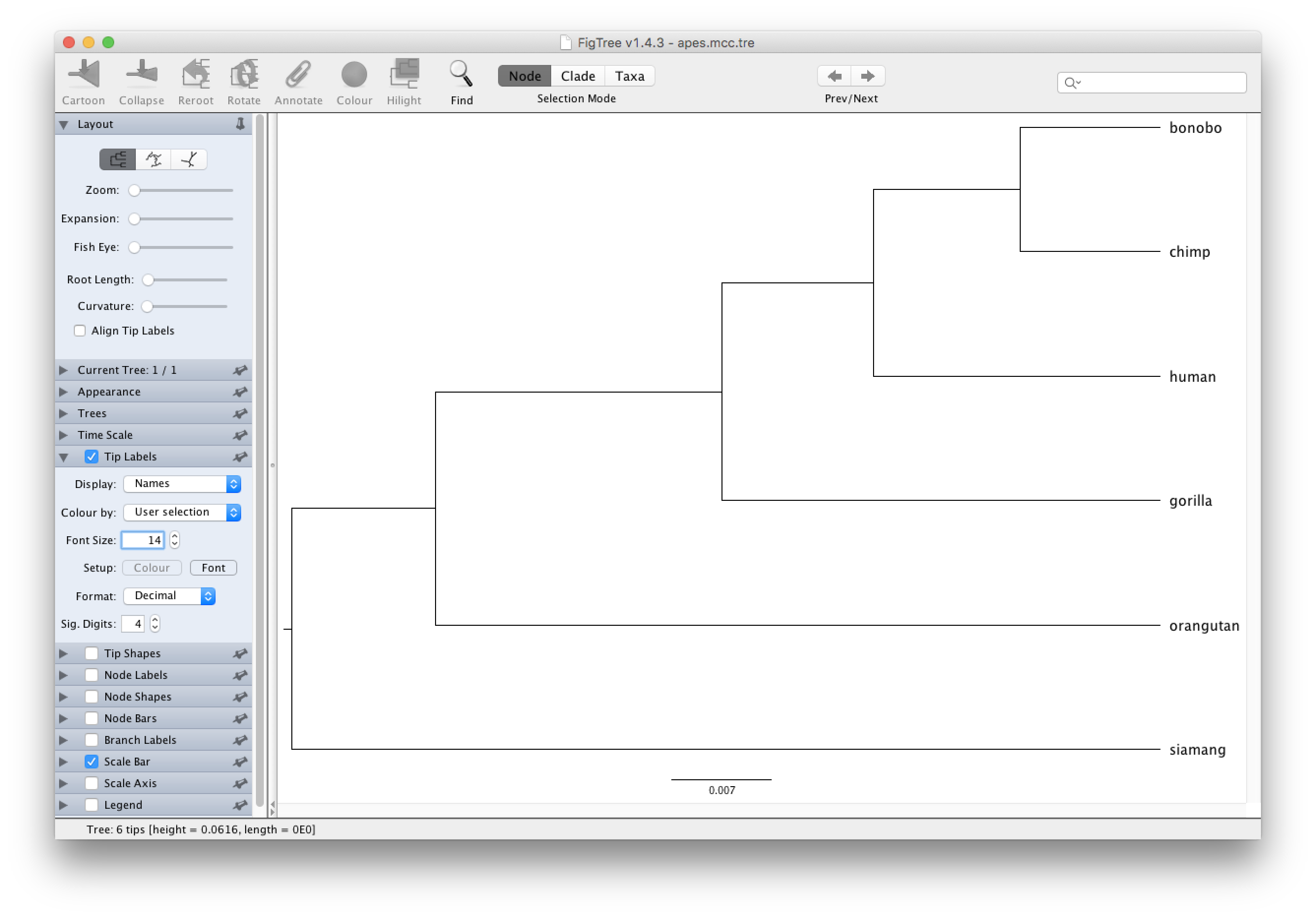
The final step is to load the constructed MCC tree into FigTree, which allows to visualise the tree and accompanying summary information produced by TreeAnnotator.
After starting FigTree, simply go to File and Open... the apes.mcc.tree file.
Typically, nodes from the tree are drawn in increasing node order (go to Tree and select Increasing Node Order to do so).
Given that we did not incorporate any timing information into our analysis, for example by providing a calibration prior, the scale beneath the tree will be expressed in average number of substitutions per time unit (and no time axis can hence be added).
Increase the font size of the tip labels by setting a Font Size of e.g. 14 in the Tip Labels section on the left hand side: