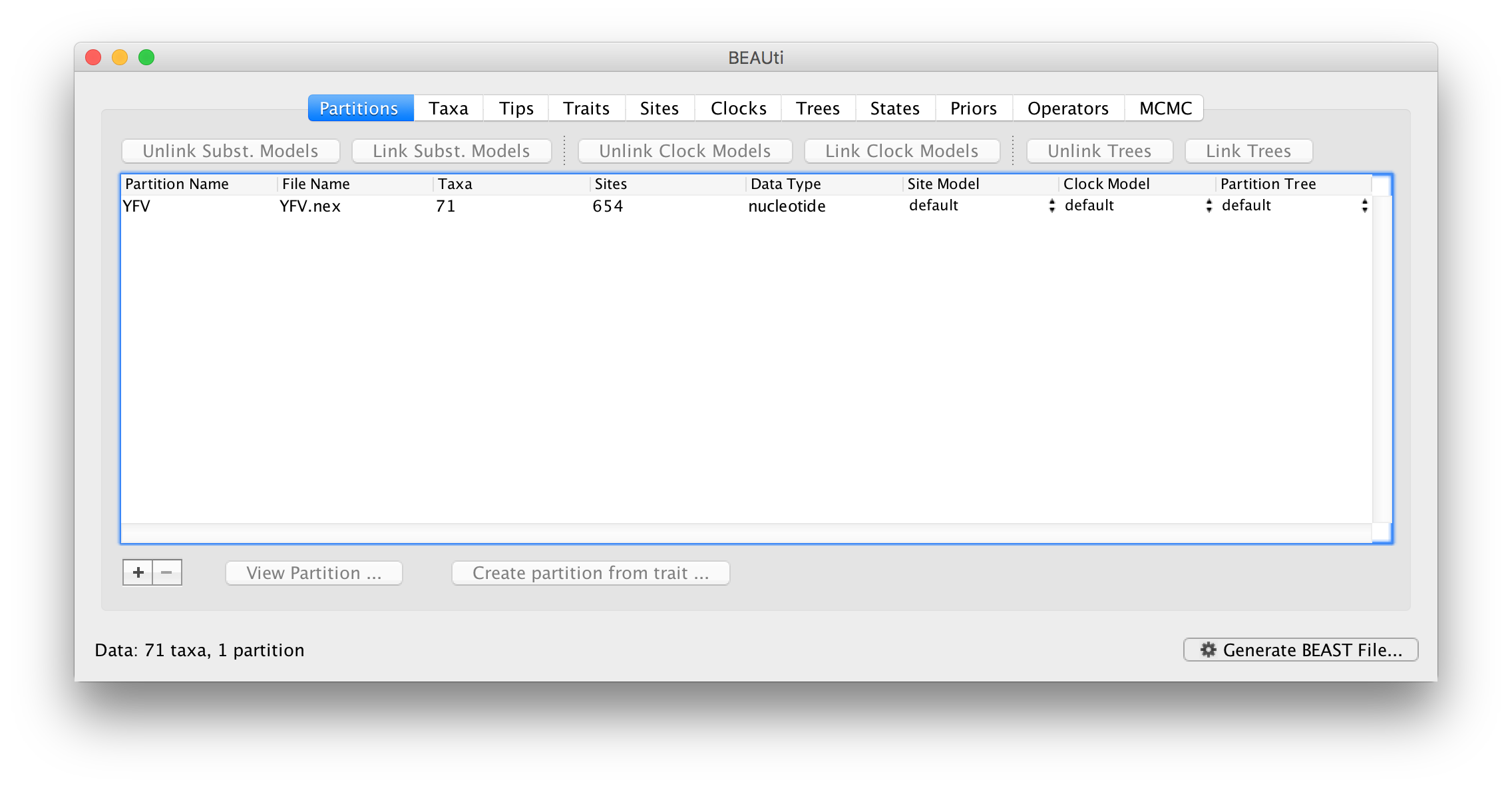
The data are 71 sequences from the prM/E gene of yellow fever virus (YFV) from Africa and the Americas with isolation dates ranging from 1940-2009. The sequences represent a subset of the data set analyzed by Bryant et al. (Bryant JE, Holmes EC, Barrett ADT, 2007 Out of Africa: A Molecular Perspective on the Introduction of Yellow Fever Virus into the Americas. PLoS Pathog 3(5): e75).
Loading the data into BEAUti
Loading the NEXUS file
To load a NEXUS format alignment, simply select the Import Data... option from the File menu and select the file called YFV.nex.
This file contains an alignment of 71 sequences from the prM/E gene of YFV, 654 nucleotides in length.
Once loaded, the sequence data will be listed under Data Partitions:
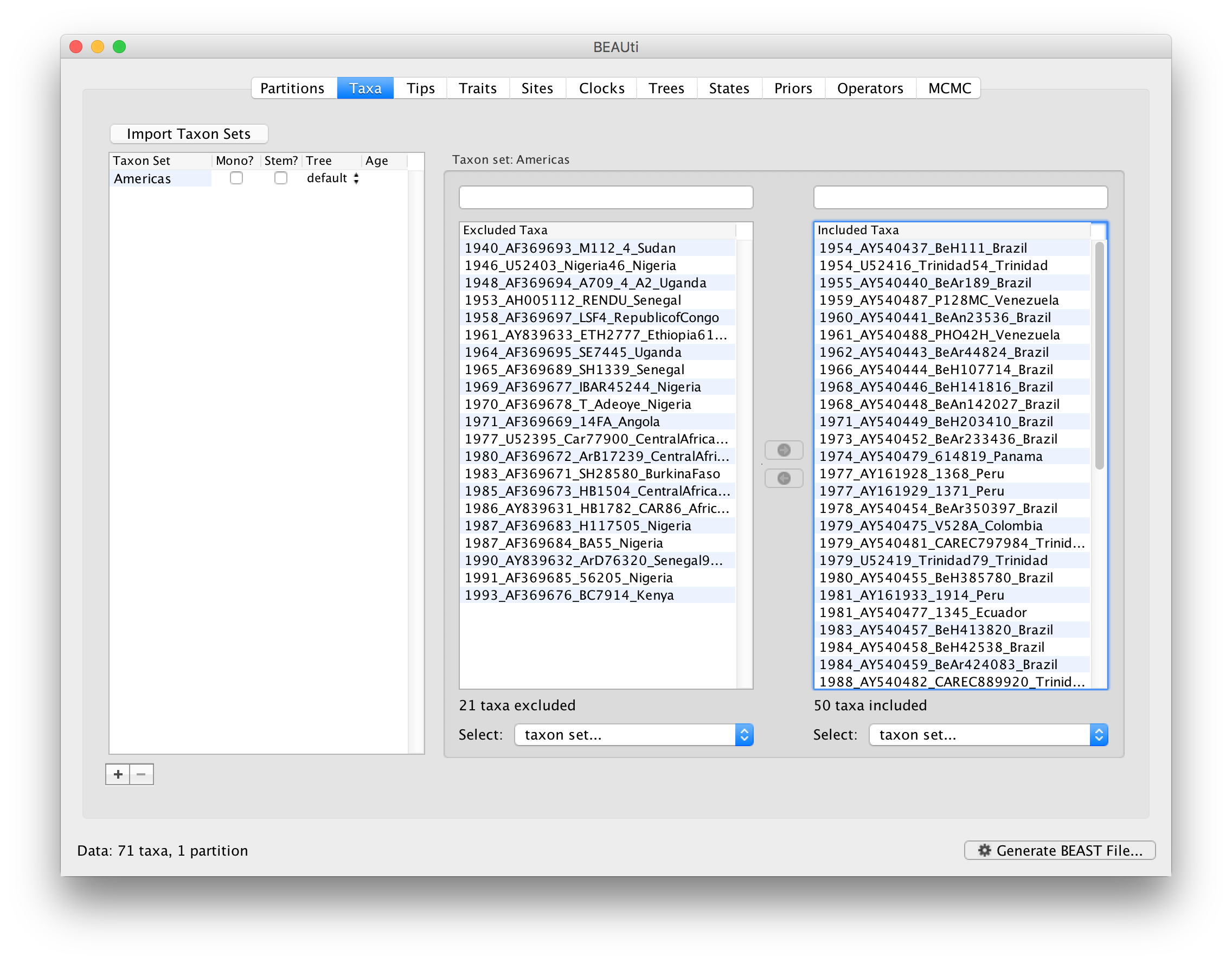
Specifying a taxon set
Under the Taxa panel, we can define sets of taxa for which we would like to obtain particular statistics, enforce a monophyletic constraint, or put calibration information on.
Let’s define an “Americas” taxon set by pressing the small “plus” button at the bottom left of the panel:
This will create a new taxon set.
Rename it by double-clicking on the entry that appears (it will initially be called untitled1).
Call it Americas.
Do not enforce monophyly using the monophyletic? option because we will evaluate the support for this cluster.
We do not opt for the includeStem? option either because we would like to estimate the TRMCA for the viruses from the Americas and not for the parent node leading to this clade.
In the next table along you will see the available taxa.
Taxa can be selected and moved to the Included taxa set by pressing the green arrow button.
Note that multiple taxa can be selected simultaneously holding down the Command or Control button on a Mac or PC, respectively.
Since most taxa are from the Americas, the most convenient is to simply select all taxa, move them to the ‘Included taxa’ set, and then move back the African taxa (the country of sampling is included at the end of the taxa names). Check there are only African countries on the left (there should be 21) and only American countries on the right (there should be 50).
For more information on creating taxon sets, see this page.
After these operations, the screen should look like this:
To inform BEAUti/BEAST about the sampling dates of the sequences, go to the Tips menu and select the “Use tip dates” option. By default all the taxa are assumed to have a date of zero (i.e. the sequences are assumed to be sampled at the same time; BEAST considers the present or most recent sampling time as time 0). In this case, the YFV sequences have been sampled at various dates going back to the 1940s. The actual year of sampling is given in the name of each taxon and we could simply edit the value in the Date column of the table to reflect these. However, if the taxa names contain the calibration information, then a convenient way to specify the dates of the sequences in BEAUti is to use the Parse Dates button at the top of the Data panel. Clicking this will make a dialog box appear:
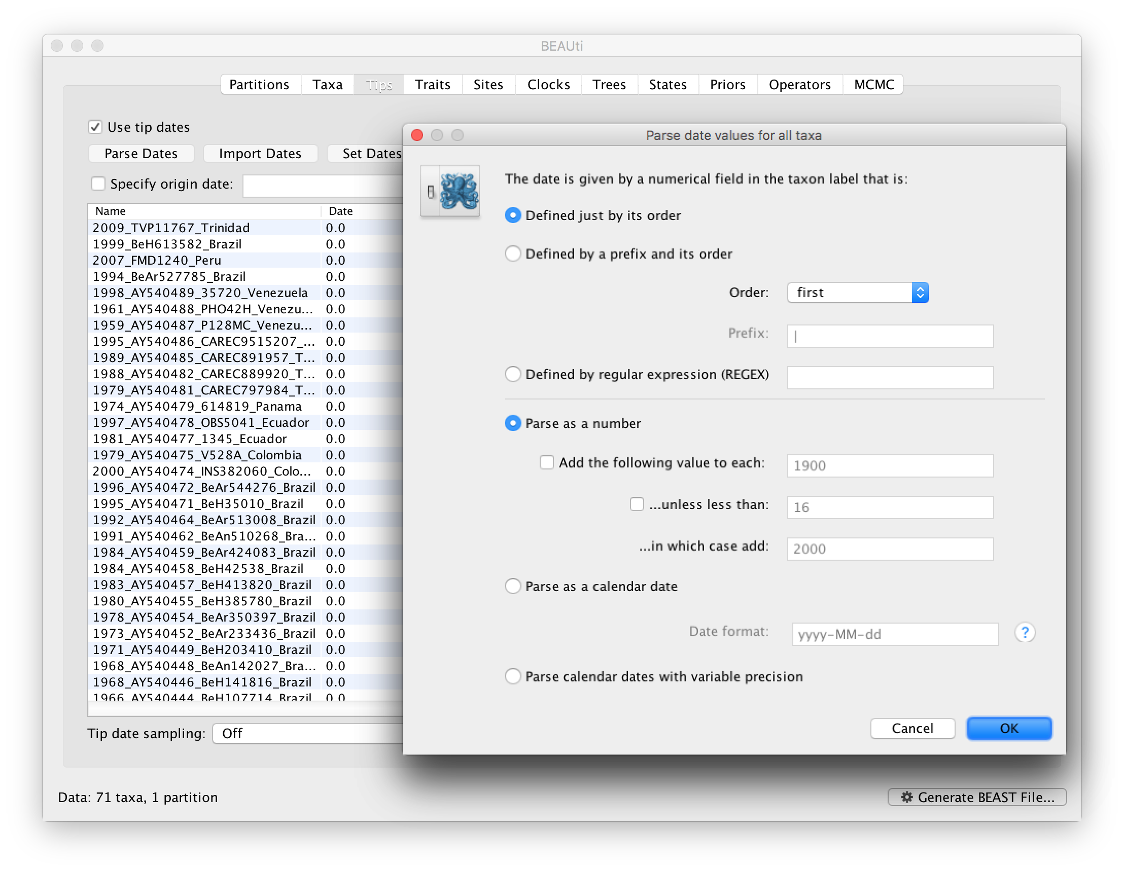
This operation attempts to guess what the dates are from information contained within the taxon names. It works by trying to find a numerical field within each name. If the taxon names contain more than one numerical field (such as the some YFV sequences, above) then you can specify how to find the one that corresponds to the date of sampling. See this page for details about the various options for setting dates in this panel. For the YFV sequences you can keep the default Defined just by its order and Order: first (but make sure that the Parse as a number option is selected).
When parsing a number, you can ask BEAUti to add a fixed value to each date which can be useful for transforming a 2 digit year into a 4 digit year. Because all dates are specified in a four digit format in this case, no additional settings are needed. So, we can press OK.
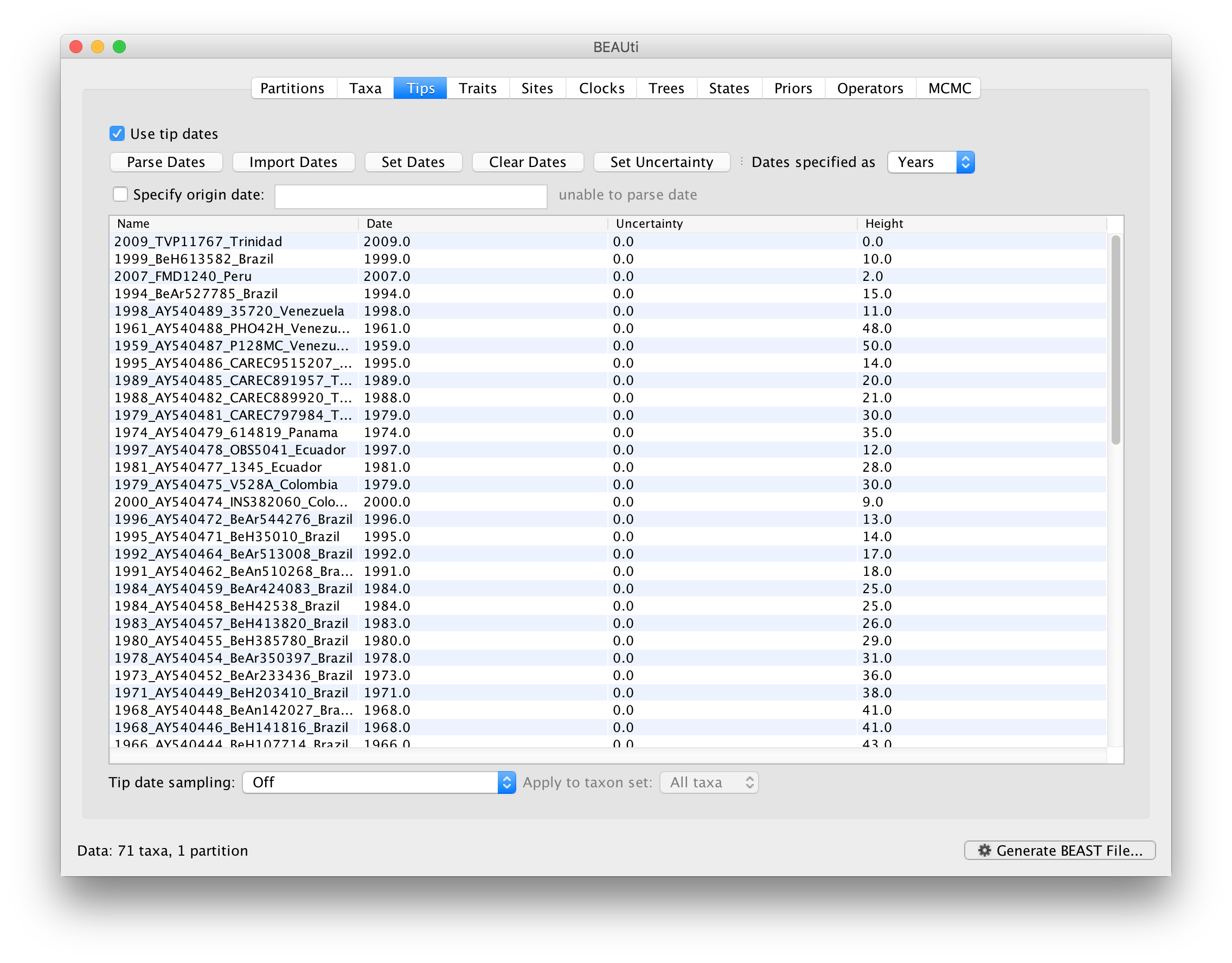
The Height column lists the ages of the tips relative to time 0 (in our case 2009). For these sequences, only the sampling year is provided and not the exact sampling dates. This uncertainty will negligible with respect to the relatively large evolutionary time scale of this example, however, it is possible to accommodate the sampling time uncertainty — see here.
Setting the evolutionary model
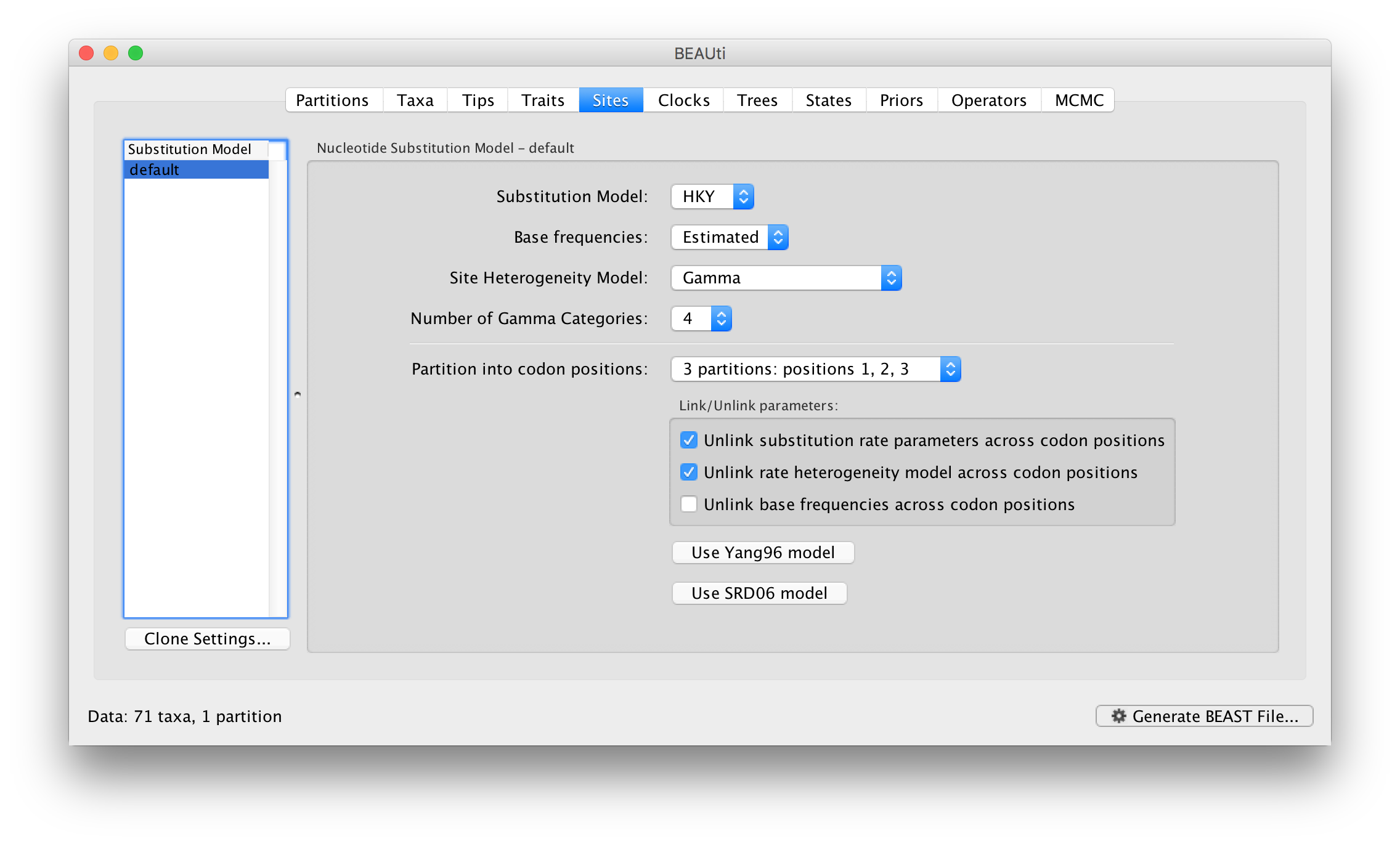
The next thing to do is to click on the Sites tab at the top of the main window. This will reveal the evolutionary model settings for BEAST. Exactly which options appear depend on whether the data are nucleotides or amino acids (or traits). This tutorial assumes that you are familiar with the evolutionary models available; however there are a couple of points to note about selecting a model in BEAUti:
- Partition into codon positions:
- Selecting the
Partition into codon positionsoption assumes that the data are aligned as codons. This option will then estimate a separate rate of substitution for each codon position, or for 1+2 versus 3, depending on the setting. - Unlink substitution model across codon positions:
- Selecting the
Unlink substitution model across codon positionswill specify that BEAST should estimate a separate transition-transversion ratio or general time reversible rate matrix for each codon position. - Unlink rate heterogeneity model across codon positions:
- Selecting the
Unlink rate heterogeneity model across codon positionswill specify that BEAST should estimate set of rate heterogeneity parameters (gamma shape parameter and/or proportion of invariant sites) for each codon position. - Unlink base frequencies across codon positions:
- Selecting the
Unlink base frequencies across codon positionswill specify that BEAST should estimate a separate set of base frequencies for each codon position.
For this tutorial, select the 3 partitions: codon positions 1, 2 & 3 option so that each codon position has its own HKY substitution model, rate of evolution, Estimated base frequencies, and Gamma-distributed rate variation among sites:
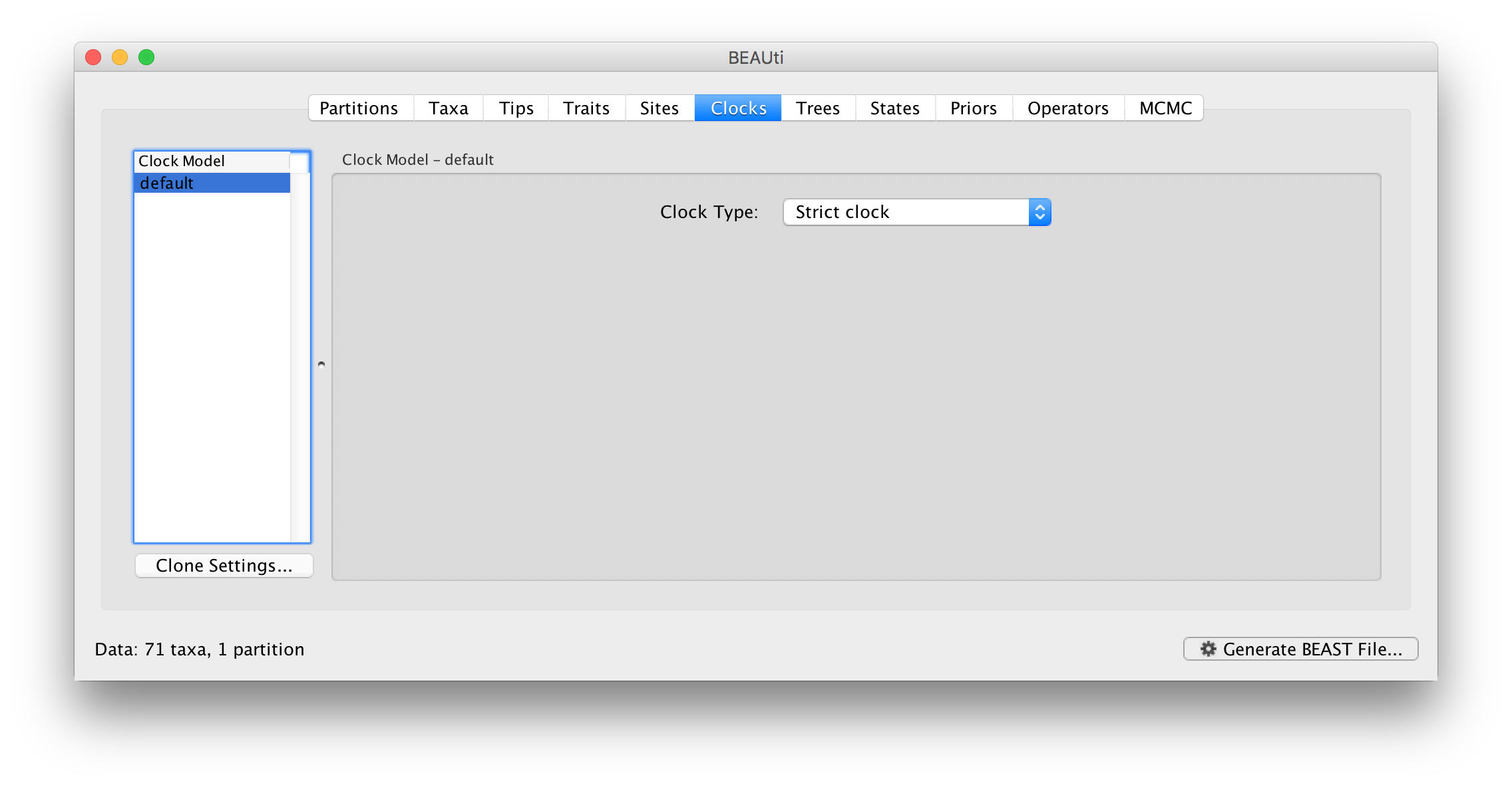
Setting the clock model
Click on the Clocks tab at the top of the main window. We will perform our initial run using the (default) strict molecular clock model:
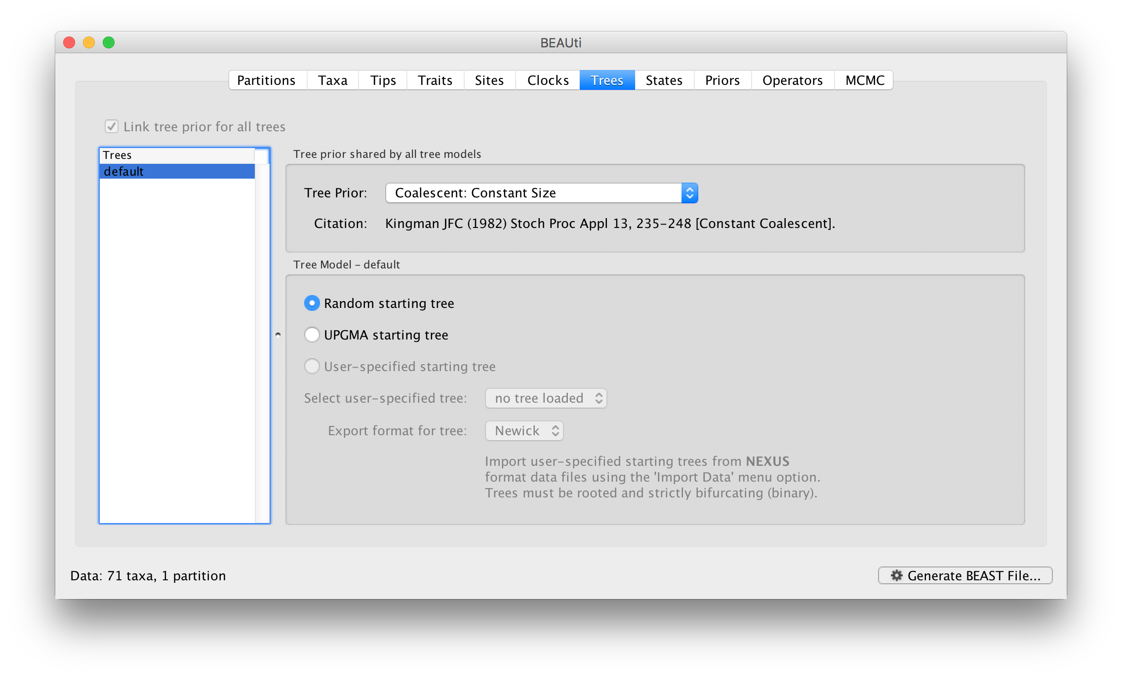
Setting the starting tree and tree prior
Click on the Trees tab at the top of the main window. We keep a default random starting tree and a (simple) constant size coalescent prior. The tree priors (coalescent and other models) are described on this page.
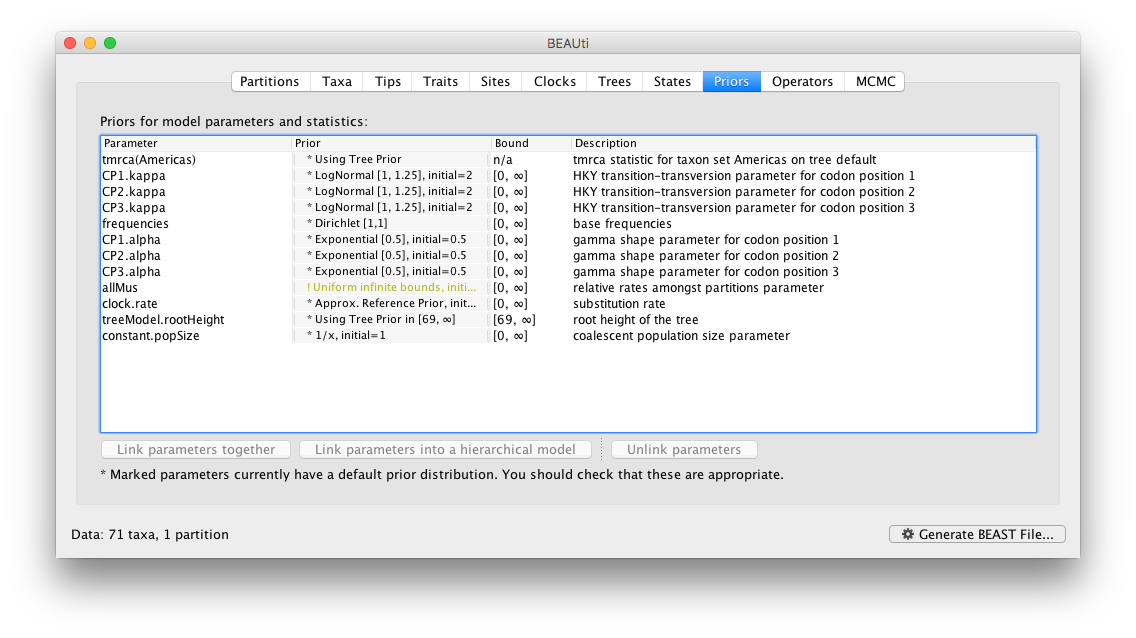
Setting up the priors
Review the prior settings under the Priors panel:
Setting up the operators
Each parameter in the model has one or more “operators” (these are variously called moves, proposals or transition kernels by other MCMC software packages such as MrBayes and LAMARC). The operators specify how the parameters change as the MCMC runs. As of BEAST v1.8.4, different options are available w.r.t. exploring tree space. In this tutorial, we will use the ‘classic operator mix’, which consists of of set of tree transition kernels that propose changes to the tree. There is also an option to fix the tree topology as well as a ‘new experimental mix’, which is currently under development with the aim to improve mixing for large phylogenetic trees.
The operators panel in BEAUti has a table that lists the parameters, their operators and the tuning settings for these operators:
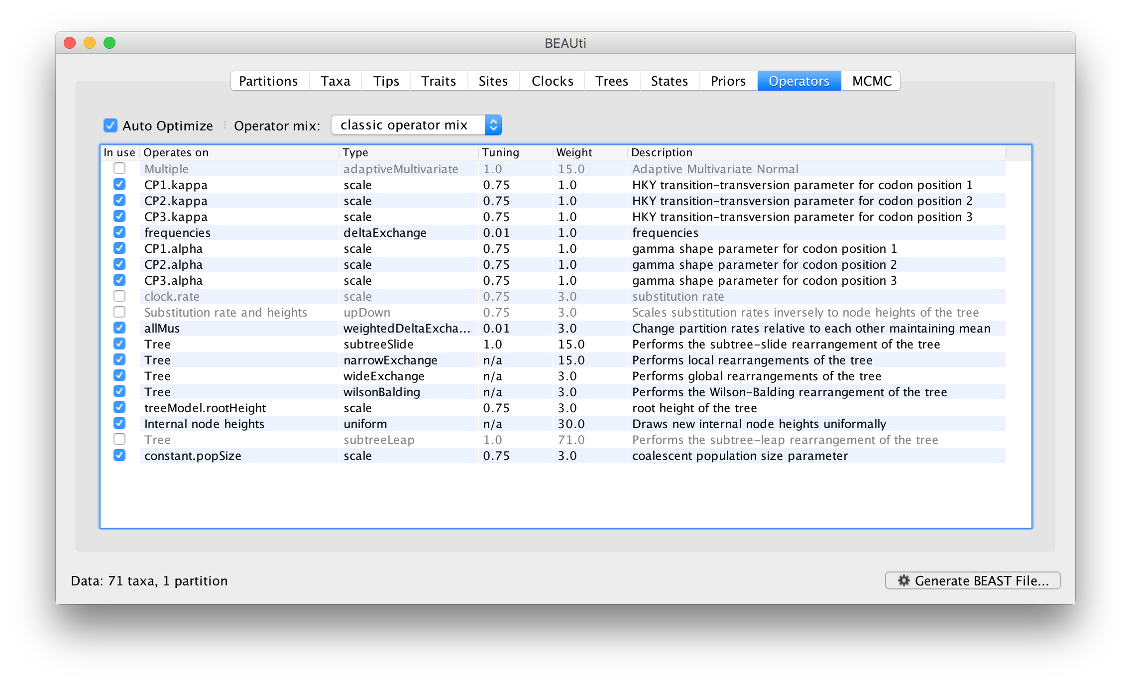
In the first column are the parameter names. These will be called things like CP1.kappa which means the HKY model’s kappa parameter (the transition-transversion bias) for the first codon position. The next column has the type of operators that are acting on each parameter. For example, the scale operator scales the parameter up or down by a random proportion and the uniform operator simply picks a new value uniformly within a range. Some parameters related to the tree or to the node ages in the tree are associated with specific operators.
The next column, labelled Tuning, gives a tuning setting to the operator. Some operators don’t have any tuning settings so have n/a under this column. The tuning parameter will determine how large a move each operator will make which will affect how often that change is accepted by the MCMC which will affect the efficiency of the analysis. For most operators (like the subtree slide operator) a larger tuning parameter means larger moves. However for the scale operator a tuning parameter value closer to 0.0 means bigger moves. At the top of the window is an option called Auto Optimize which, when selected, will automatically adjust the tuning setting as the MCMC runs to try to achieve maximum efficiency. At the end of the run a table of the operators, their performance and the final values of these tuning settings can be written to standard output.
The next column, labelled Weight, specifies how often each operator is applied relative to the others. Some parameters tend to be sampled very efficiently from their target distribution (e.g. the kappa parameter); these parameters can have their operators down-weighted so that they are not changed as often. We will start by using the default settings for this analysis.
Setting the MCMC options
The MCMC tab in BEAUti provides settings to control the MCMC chain. Firstly we have the Length of chain. This is the number of steps the MCMC will make in the chain before finishing. How long this should depend on the size of the dataset, the complexity of the model and the precision of the answer required. The default value of 10,000,000 is entirely arbitrary and should be adjusted according to the size of your dataset. We will see later how the resulting log file can be analyzed using Tracer in order to examine whether a particular chain length is adequate.
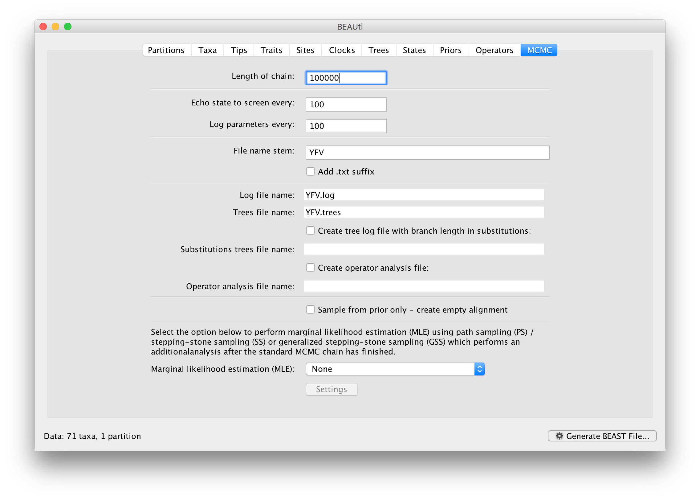
The next couple of options specify how often the current parameter values should be displayed on the screen and recorded in the log file. The screen output is simply for monitoring the program’s progress so can be set to any value (although if set too small, the sheer quantity of information being displayed on the screen will slow the program down). For the log file, the value should be set relative to the total length of the chain. Sampling too often will result in very large files with little extra benefit in terms of the precision of the estimates. Sample too infrequently and the log file will not contain much information about the distributions of the parameters. You probably want to aim to store no more than 10,000 samples so this should be set to something >= chain length / 10,000.
For this dataset let’s initially set the chain length to 100,000 as this will run reasonably quickly on most modern computers. Although the suggestion above would indicate a lower sampling frequency, in this case set both the sampling frequencies to 100. The next option allows the user to set the File stem name; if not set to ‘YFV’ by default, you can type this in here. The next two options give the file names of the log files for the parameters and the trees. These will be set to a default based on the file stem name. Let’s also create an operator analysis file by selecting the relevant option. An option is also available to sample from the prior only, which can be useful to evaluate how divergent our posterior estimates are when information is drawn from the data. Here, we will not select this option, but analyze the actual data. Finally, one can select to perform marginal likelihood estimation to assess model fit; we will return to this later in this tutorial.
At this point we are ready to generate a BEAST XML file and to use this to run the Bayesian evolutionary analysis. To do this, either select the Generate BEAST File… option from the File menu or click the similarly labelled button at the bottom of the window. BEAUti will ask you to review the prior settings one more time before saving the file (and indicate that some are improper). Continue and choose a name for the file (for example, YFV.xml) and save the file.
For convenience, leave the BEAUti window open so that you can change the values and re-generate the BEAST file as required later in this tutorial.
Running BEAST
Once the BEAST XML file has been created the analysis itself can be performed using BEAST. The exact instructions for running BEAST depends on the computer you are using, but in most cases a standard file dialog box will appear in which you select the XML file: If the command line version is being used then the name of the XML file is given after the name of the BEAST executable. When you have installed the BEAGLE library (code.google.com/p/beagle-lib/), you can use this in conjunction with BEAST to speed up the calculations. If not installed, unselect the use of the BEAGLE library. When pressing “Run”, the analysis will be performed with detailed information about the progress of the run being written to the screen. When it has finished, the log file and the trees file will have been created in the same location as your XML file.
Analysing the BEAST output
To analyze the results of running BEAST we are going to use the program Tracer. The exact instructions for running Tracer differs depending on which computer you are using. Please see the README text file that was distributed with the version you downloaded. Once running, Tracer will look similar irrespective of which computer system it is running on.
Select the Import Trace File... option from the File menu. If you have it available, select the log file that you created in the previous section. The file will load and you will be presented with a window similar to the one below. Remember that MCMC is a stochastic algorithm so the actual numbers will not be exactly the same.
On the left hand side is the name of the log file loaded and the traces that it contains. There are traces for a quantity proportional to posterior (this is the product of the data likelihood and the prior probabilities, on the log-scale), and the continuous parameters. Selecting a trace on the left brings up analyses for this trace on the right hand side depending on tab that is selected. When first opened, the posterior trace is selected and various statistics of this trace are shown under the Estimates tab.
In the top right of the window is a table of calculated statistics for the selected trace. The statistics and their meaning are described in the table below.
- Mean
- The mean value of the samples (excluding the burn-in).
- Stdev of mean
- The standard error of the mean. This takes into account the effective sample size so a small ESS will give a large standard error.
- Median
- The median value of the samples (excluding the burn-in).
- Geometric mean
- The central tendency or typical value of the set of samples (excluding the burn-in).
- 95% HPD Lower
- The lower bound of the highest posterior density (HPD) interval. The HPD is the shortest interval that contains 95% of the sampled values.
- 95% HPD Upper
- The upper bound of the highest posterior density (HPD) interval.
- Auto-Correlation Time (ACT)
- The average number of states in the MCMC chain that two samples have to be separated by for them to be uncorrelated (i.e. independent samples from the posterior). The ACT is estimated from the samples in the trace (excluding the burn-in).
- Effective Sample Size (ESS)
- The effective sample size (ESS) is the number of independent samples that the trace is equivalent to. This is calculated as the chain length (excluding the burn-in) divided by the ACT.
Note that the effective sample sizes (ESSs) for all the traces are small (ESSs less than 100 are highlighted in red by Tracer and values > 100 but < 200 are in yellow). This is not good. A low ESS means that the trace contained a lot of correlated samples and thus may not represent the posterior distribution well. In the bottom right of the window is a frequency plot of the samples which is expected given the low ESSs is extremely rough. If we select the tab on the right-hand-side labelled `Trace’ we can view the raw trace, that is, the sampled values against the step in the MCMC chain. Here you can see how the samples are correlated. There are 1000 samples in the trace (we ran the MCMC for 100,000 steps sampling every 100) but it is clear that adjacent samples often tend to have similar values. The ESS for the age of the root (treeModel.rootHeight is about 6 so we are only getting 1 independent sample to every 167 actual samples). It also seems that the default burn-in of 10% of the chain length is inadequate (the posterior values are still increasing over most of the chain). Not excluding enough of the start of the chain as burn-in will bias the results and render estimates of ESS unreliable. The simple response to this situation is that we need to run the chain for longer. Go back to the MCMC Options section, above, and create a new BEAST XML file with a longer chain length (e.g. 10.000.000). To continue the tutorial without having to wait for a long run to complete, you can make use of the log files provided with this tutorial (chain length of 20.000.000 and logged every 10,000 sample). Import the log file for the strict clock analysis and click on the Trace tab and look at the raw trace plot.
The log file provided contains 2000 samples and with an ESS of 262 for the clock.rate there is still some degree of auto-correlation between the samples but 262 effectively independent samples will now provide an reasonable estimate of the posterior distribution. There are no obvious trends in the plot which would suggest that the MCMC has not yet converged, and there are no large-scale fluctuations in the trace which would suggest poor mixing. As we are happy with the behavior of posterior probability we can now move on to one of the parameters of interest: substitution rate. Select clock.rate in the left-hand table. This is the average substitution rate across all sites in the alignment. Now choose the density plot by selecting the tab labeled Marginal Prob Distribution. This plot shows a kernel density estimate (KDE) of the posterior probability density of this parameter. You should see a plot similar to this:
As you can see the posterior probability density is nicely bell-shaped. When looking at the equivalent histogram in the Estimates panel, there is some sampling noise which is smoothened by the KDE; this would be reduced if we ran the chain for longer but we already have a reasonable estimate of the mean and HPD interval. You can overlay the density plots of multiple traces in order to compare them (it is up to the user to determine whether they are comparable on the the same axis or not). Select the relative substitution rates for all three codon positions in the table to the left (labelled CP1.mu, CP2.mu and CP3.mu and select ‘Top-Right’ under Legend. This will show the posterior probability densities for the relative substitution rate at all three codon positions overlaid:
Note that the three rates are markedly different, what does this tell us about the selective pressure on this gene? Now, let’s have a look at the time to the most recent common ancestor (tmrca) for the strains from the Americas relative to the general tmrca:
This indicates that the tmrca for the Americas is significantly younger than the root height and argues for more recent origin of YFV in the Americas.
Summarizing the trees
We have seen how we can diagnose our MCMC run using Tracer and produce estimates of the marginal posterior distributions of parameters of our model. However, BEAST also samples trees (either phylogenies or genealogies) at the same time as the other parameters of the model. These are written to a separate file called the `trees’ file. This file is a standard NEXUS format file. As such it can easily be loaded into other software in order to examine the trees it contains. One possibility is to load the trees into a program such as PAUP* and construct a consensus tree in a similar manner to summarizing a set of bootstrap trees. In this case, the support values reported for the resolved nodes in the consensus tree will be the posterior probability of those clades.
In this tutorial, however, we are going to use a tool that is provided as part of the BEAST package to summarize the information contained within our sampled trees. The tool is called TreeAnnotator and once running, you will be presented with a window like the one below.
TreeAnnotator takes a single `target’ tree and annotates it with the summarized information from the entire sample of trees. The summarized information includes the average node ages (along with the HPD intervals), the posterior support and the average rate of evolution on each branch (for models where this can vary). The program calculates these values for each node or clade observed in the specified ‘target’ tree. Burnin - This is either the number of states or the number of trees in the input file that should be excluded from the summarization. This value is given as the number of trees rather than the number of steps in the MCMC chain. Thus for the example above, with a chain of 20,000,000 steps, a burn-in of 10% as the number of states can be specified as 2,000,000 states. Alternatively, with a chain of 20,000,000 steps, sampling every 10000 steps, there are 2000 trees in the file. To obtain a 10% burnin, set the burnin as the number of trees value to 200. Posterior probability limit - This is the minimum posterior probability for a node in order for TreeAnnotator to store the annotated information. Keep this value to the default of 0.0 to summarize all nodes in the target tree. Target tree type - This has two options “Maximum clade credibility” or “User target tree”. For the latter option, a NEXUS tree file can be specified as the Target Tree File, below. For the former option, TreeAnnotator will examine every tree in the Input Tree File and select the tree that has the highest product of the posterior probabilities of all its nodes.
Node heights -This option specifies what node heights (times) should be used for the output tree. If the ’Keep target heights’ is selected, then the node heights will be the same as the target tree. Node heights can also be summarised as a Mean or a Median over the sample of trees. Sometimes a mean or median height for a node may actually be higher than the mean or median height of its parental node (because particular ancestral-descendent relationships in the MCC tree may still be different compared to a large number of other tree sampled). This will result in artifactual negative branch lengths, but can be avoided by the ‘Common Ancestor heights’ option. Let’s use the default Median heights for our summary tree.
Target Tree File - If the “User target tree” option is selected then you can use “Choose File…” to select a NEXUS file containing the target tree.
Input Tree File - Use the “Choose File…” button to select an input trees file. This will be the trees file produced by BEAST. Output File - Select a name for the output tree file (e.g., YFV.MCC.tre).
Once you have selected all the options above, press the “Run” button. TreeAnnotator will analyze the input tree file and write the summary tree to the file you specified. This tree is in standard NEXUS tree file format so may be loaded into any tree drawing package that supports this. However, it also contains additional information that can only be displayed using the FigTree program.
Viewing the annotated tree
Run FigTree now and select the Open… command from the File menu. Select the tree file you created using TreeAnnotator in the previous section. The tree will be displayed in the FigTree window. On the left hand side of the window are the options and settings which control how the tree is displayed. In this case we want to display the posterior probabilities of each of the clades present in the tree and estimates of the age of each node. In order to do this you need to change some of the settings.
First, re-order the node order by Increasing Node Order under the Tree Menu. Click on Branch Labels in the control panel on the left and open its section by clicking on the arrow on the left. Now select posterior under the Display option. The relative magnitude of such annotations can also be represented by node shapes.
We can also plot a time scale axis for this evolutionary history (select ‘Scale Axis’ and deselect ‘Scale bar’). For appropriate scaling, open the ‘Time Scale’ section of the control panel, set the ‘Offset’ to 2009.0, the scale factor to -1.0. and ‘Reverse Axis’ under ‘Scale Axis’.
Finally, open the Appearance panel and alter the Line Weight to draw the tree with thicker lines. You can also color clades by selecting a branch, select the ‘Clade’ selection mode and choose a color. None of the options actually alter the tree’s topology or branch lengths in anyway so feel free to explore the options and settings (Highlight or collapse for example the Americas clade). You can also save the tree and this will save most of your settings so that when you load it into FigTree again it will be displayed almost exactly as you selected. The tree can also be exported to a graphics file (pdf, eps, etc.). How do the viruses from the Americas cluster relative to the African viruses and what conclusions can we draw from the inferred time scale?