Identifying convergence problems using Tracer
In a previous tutorial, analysing the output of a standard BEAST analysis using Tracer 1.7 was discussed. Here, this tutorial is extended towards analysing multiple independent runs (using the same combination of models), using different starting seeds (which leads to different random draws for all parameters involved to act as the initial estimates), in Tracer 1.7.
Data set information
Here, we take a look at an analysis of a (n unpublished) simulated data set based on a hepatitis C virus (HCV) data set, which consists of 378 taxa sampled between 1965 and July 2012. Two independent BEAST analyses (i.e. analysing the same simulated data set but with different starting seeds) were performed on this simulated data set, each comprising 90 million iterations, and should hence converge to the same posterior distribution. Comparison of marginal distributions and/or traces from multiple replicate chains can assist in diagnosing problems with phylogenetic MCMC analyses, given that well-behaved replicate chains will lead to similar posterior distributions.
Loading output files into Tracer
We start by loading the output .log files of both replicates of the same BEAST XML into Tracer 1.7. To load the log file(s), select the Open option from the File menu or drag and drop the log file into the Tracer window. The files will load and you will be presented with a window similar to the one below.
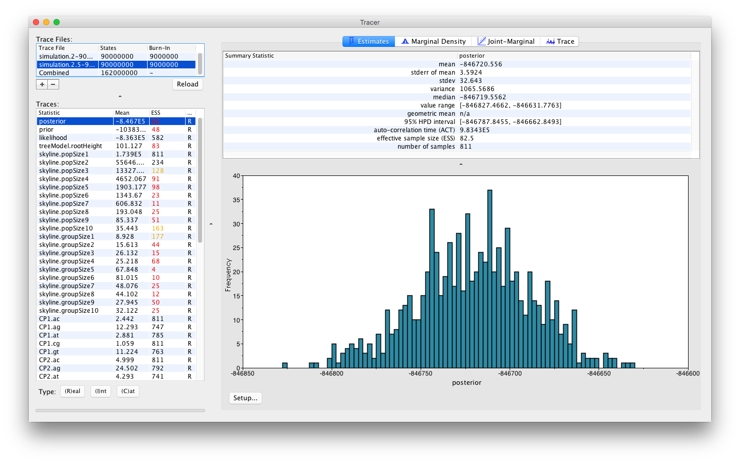
As with loading a single log file, the name of the log file loaded and the traces that it contains can be seen on the left hand side. When the different files loaded contain the same set of logged parameters, then a Combined trace will automatically appear (with a number of iterations equal to the sum of the two traces minus their burn-in length).
Exploring combined traces
Selecting the Combined trace allows to explore a concatenation of the log files. For the example we’re exploring here, selecting the Combined trace will yield the following visualisation:
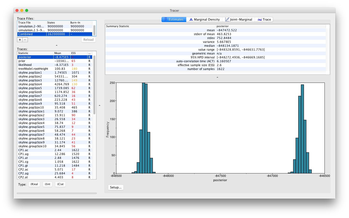
The histogram shown indicates a clear problem with the analysis, as the distribution of the joint density (or posterior) is bimodal. To obtain a better understanding of what’s going on, we can select the Trace panel which will show the following combined trace:
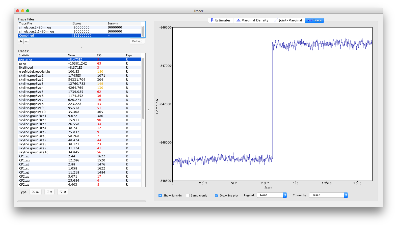
One of the joint density (or posterior) traces has converged around -848250, while the other has converged around -846750. This clearly showcases the need to perform multiple independent replicates of a Bayesian analysis, in order to be able to spot these types of problems.
Comparing individual traces
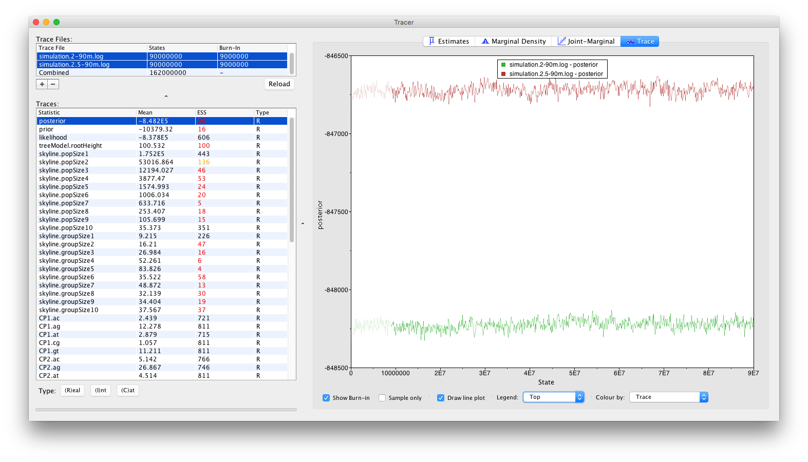
A more visually appealing approach to diagnose convergence problems is to not inspect the Combined trace, but rather inspecting the individual traces simultaneously. To this end, select the two trace files rather than the combined trace, which will generate the visualisation below. Select ‘Top’ in the Legend combo box at the bottom of the window to identify which trace belongs to which log file.
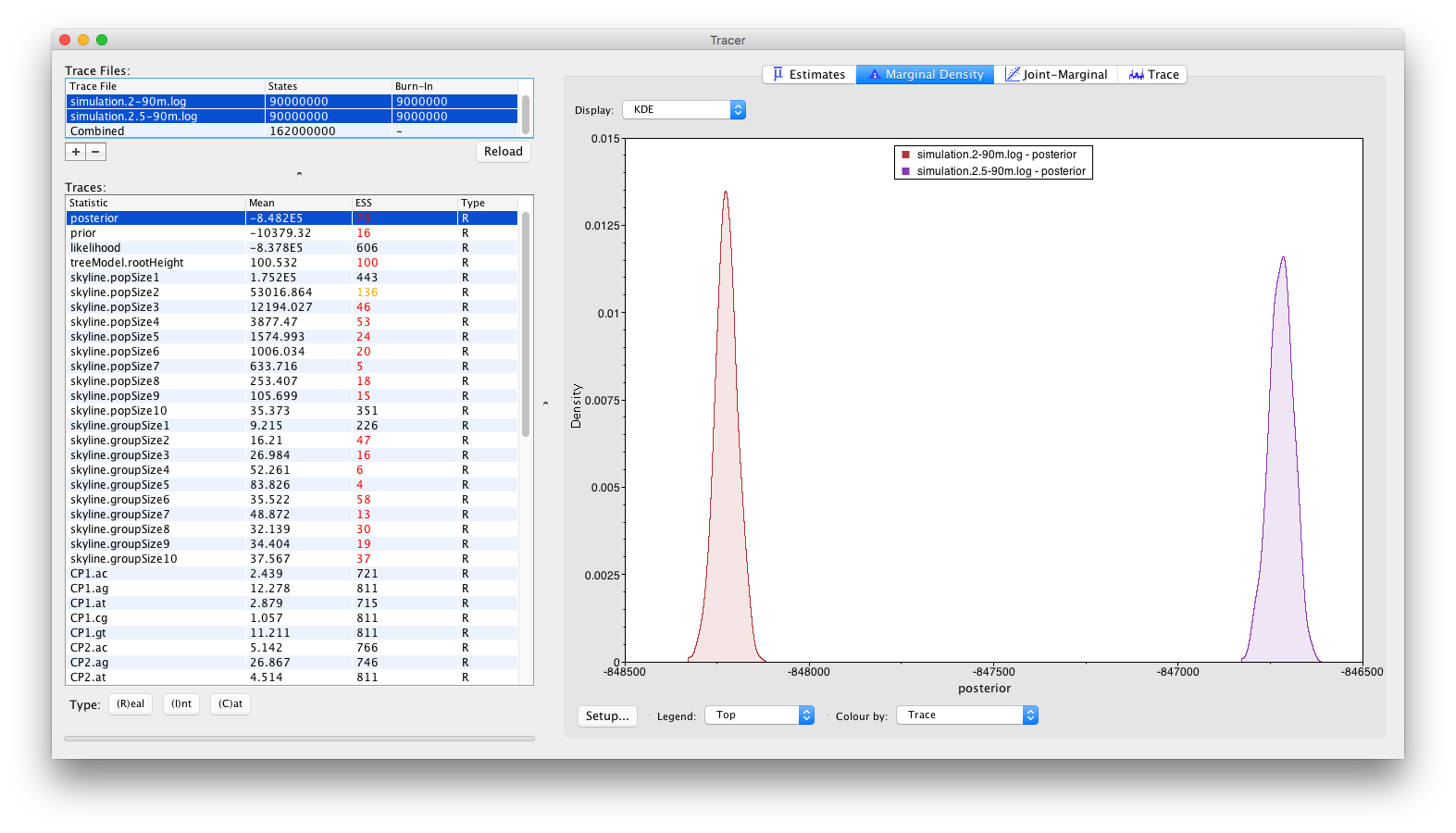
Alternative visualisations can be obtained by inspecting the Marginal Density panel:
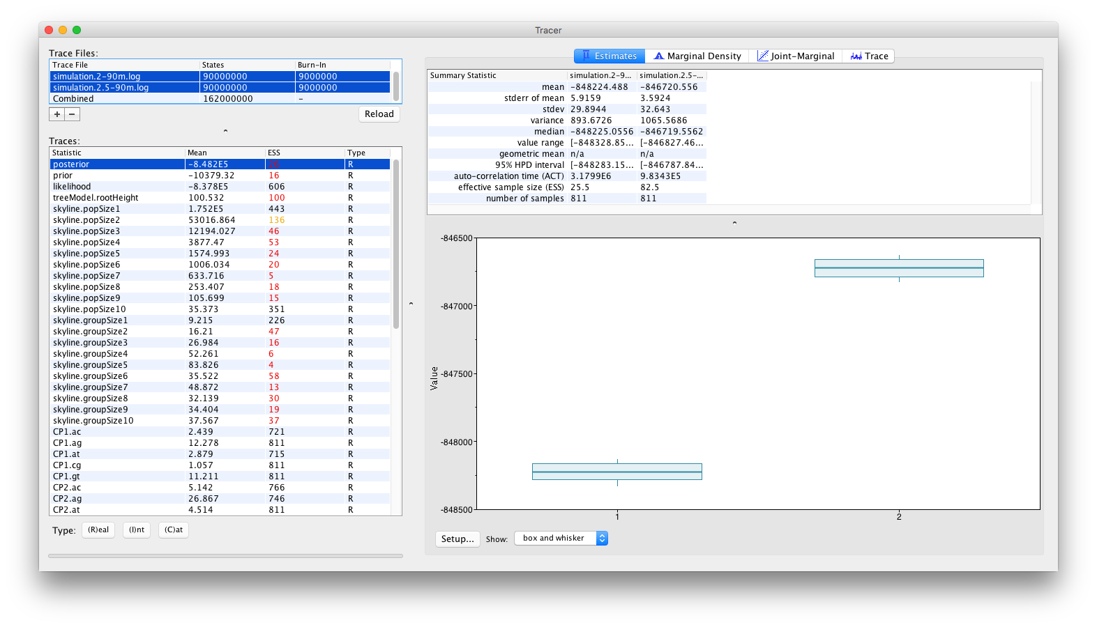
and by inspecting the Estimates panel, which allows to visualise/summarize the parameter values as either classical box plots:
or as violin plots:
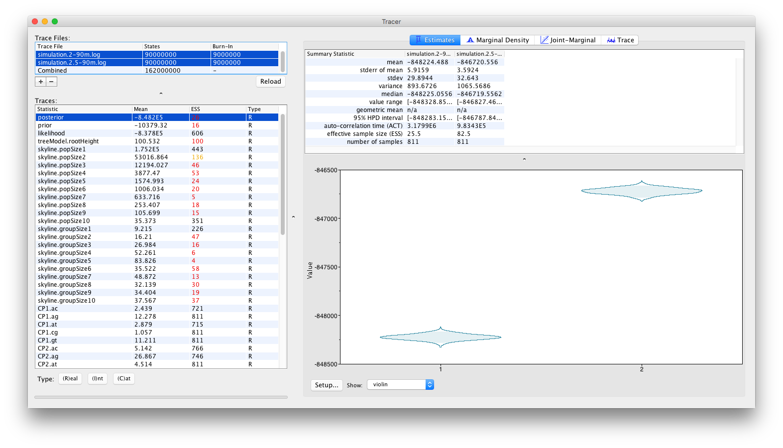
From these visualisations, it can clearly be concluded that after running for 90 million iterations, there is no sign of the replicate analyses to converge to the same joint density (or posterior). Obviously, with the current state of the analyses, no conclusions can be drawn as to which of these log files (if either) contain samples from the correct joint density. These types of convergence problems can be solved by a number of different approaches. The most obvious proposed solution would be to run the analyses for longer, in the hope that both replicate analyses convergence to the same joint density. Alternatively, it can be argued that both analyses are stuck in different (possibly local) optima and that the transition kernels need to be adjusted so that the Markov chains can escape these local optima. For example, a transition kernel that occasionally proposes a large jump across parameter space for one or more parameters may allow these analyses to converge towards the same joint density. In order to identify for which parameters this would be useful, careful inspection of the different parameter traces may be useful (to check which parameters clearly differ in their posterior estimates or if one or more parameters differ between replicate analyses).
Identifying convergence problems using TreeTracer
Data set information
We here take a look at the BEAST output of a 2020 phylogeographic study of the spread of HIV-1 subtype B in the USA (Hong et al., 2020). We focus on a data set consisting of 500 sequences that was constructed with the aim of maximizing phylogenetic diversity. The output of the original analysis consists of 1000 posterior sample trees, resulting from concatenating and downsampling two analysis replicates (i.e., the same BEAST XML was run twice, each time with a different starting seed).
What the output looks like in Tracer
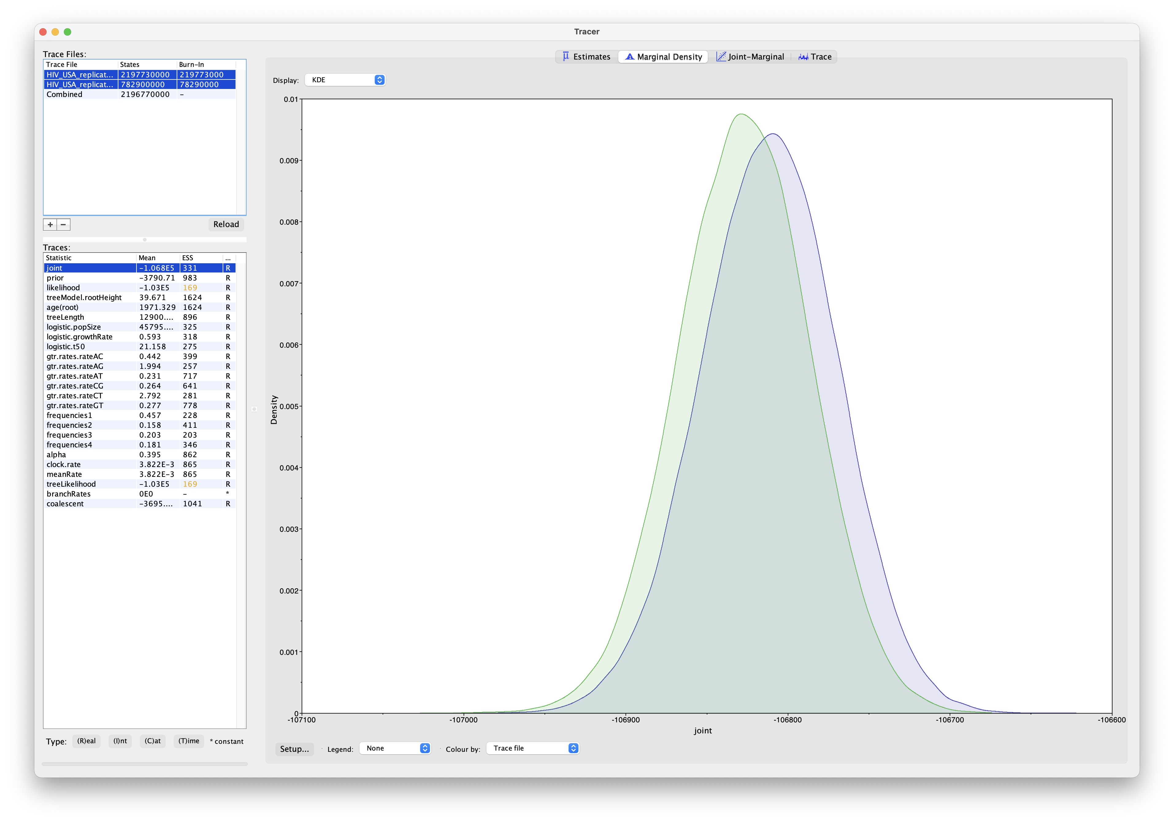
We start by loading the output .log files of both replicates (i.e. files HIV_USA_replicate_1.log and HIV_USA_replicate_2.log) of the same BEAST XML into Tracer. Inspecting the Trace panel seems to indicate that both replicates have converged to the same posterior:
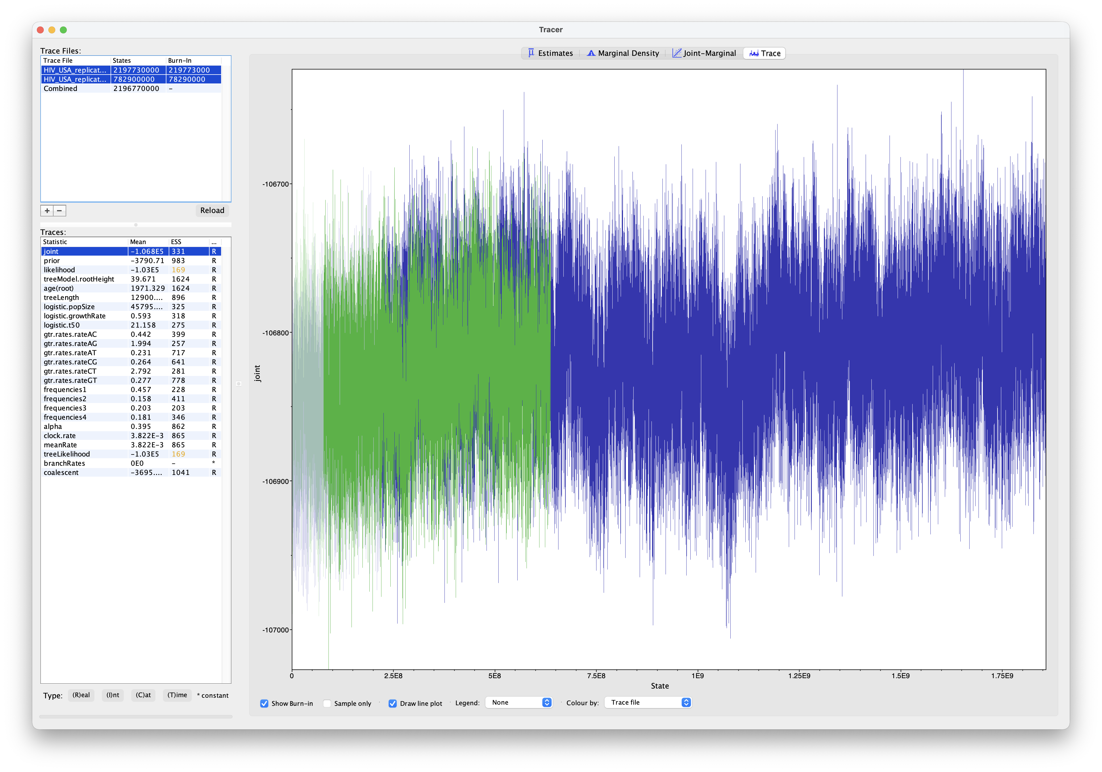
Inspecting the Marginal Density panel does point to a somewhat different posterior region being reached by both replicates. However, if you were to look at the ESS values for the combined traces, you would see that the combined ESS values are higher than for the individual replicates. Hence, when it comes to inspecting the continuous parameters in Tracer, we are likely to conclude that our two replicate analyses have converged to the same posterior.
Loading output files into TreeTracer
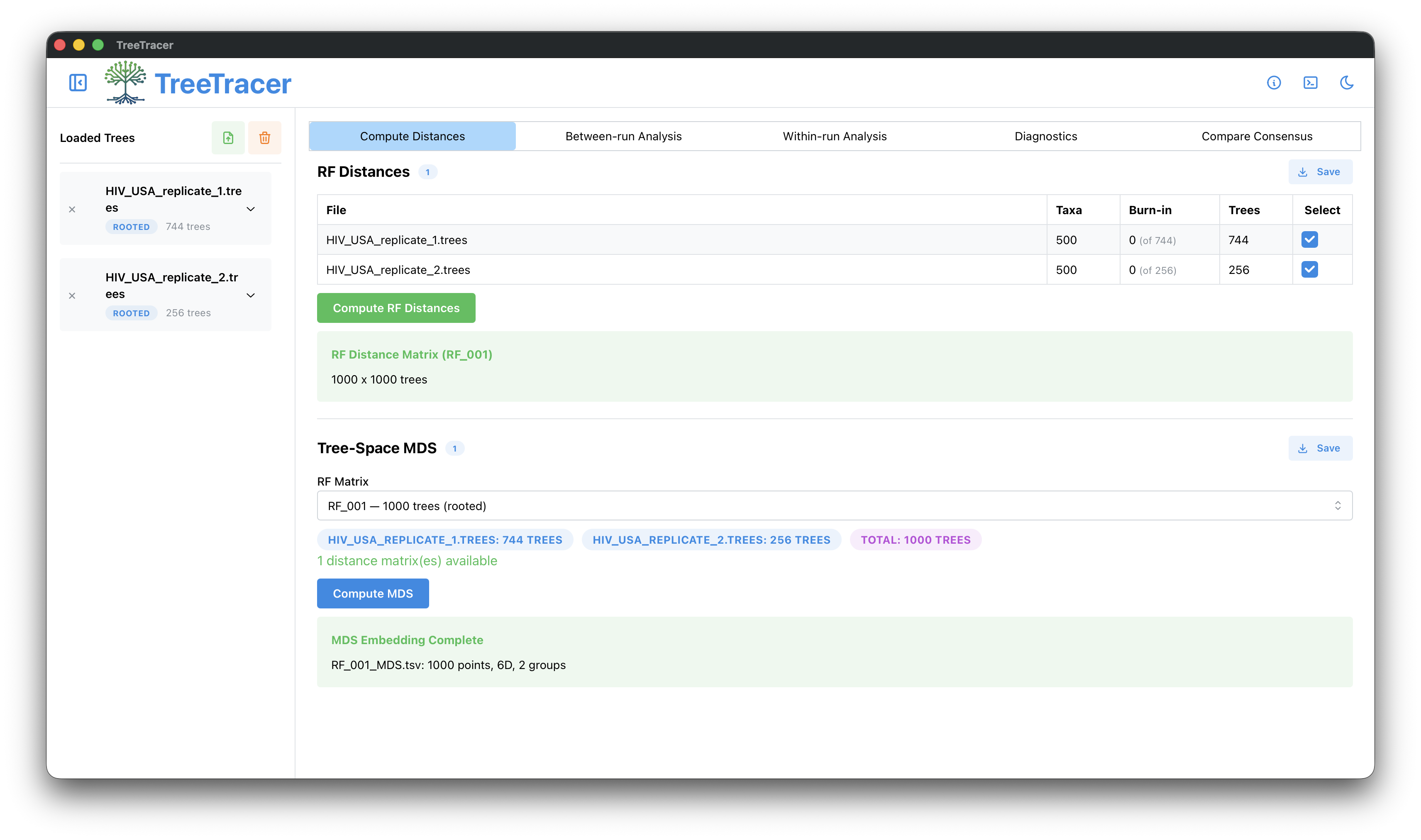
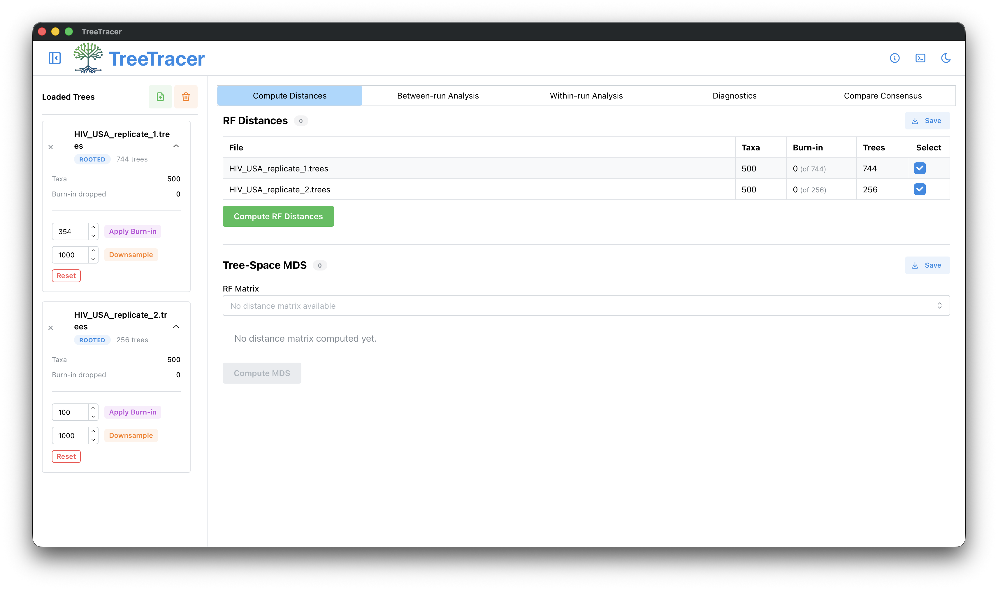
We continue with loading the output .trees files of both replicates (i.e. files HIV_USA_replicate_1.trees and HIV_USA_replicate_2.trees) of the same BEAST XML into TreeTracer. Note that far fewer samples were kept in these files compared to the .log files, as .trees files can quickly take up a lot of storage space. Given that previous publications (Hong et al., 2020; Brusselmans et al., 2024) mention that the burn-in was already discarded from the posterior sample trees files, we start our assessment in TreeTracer without any burn-in, and click the Computer RF distances and Compute MDS buttons one after the other:
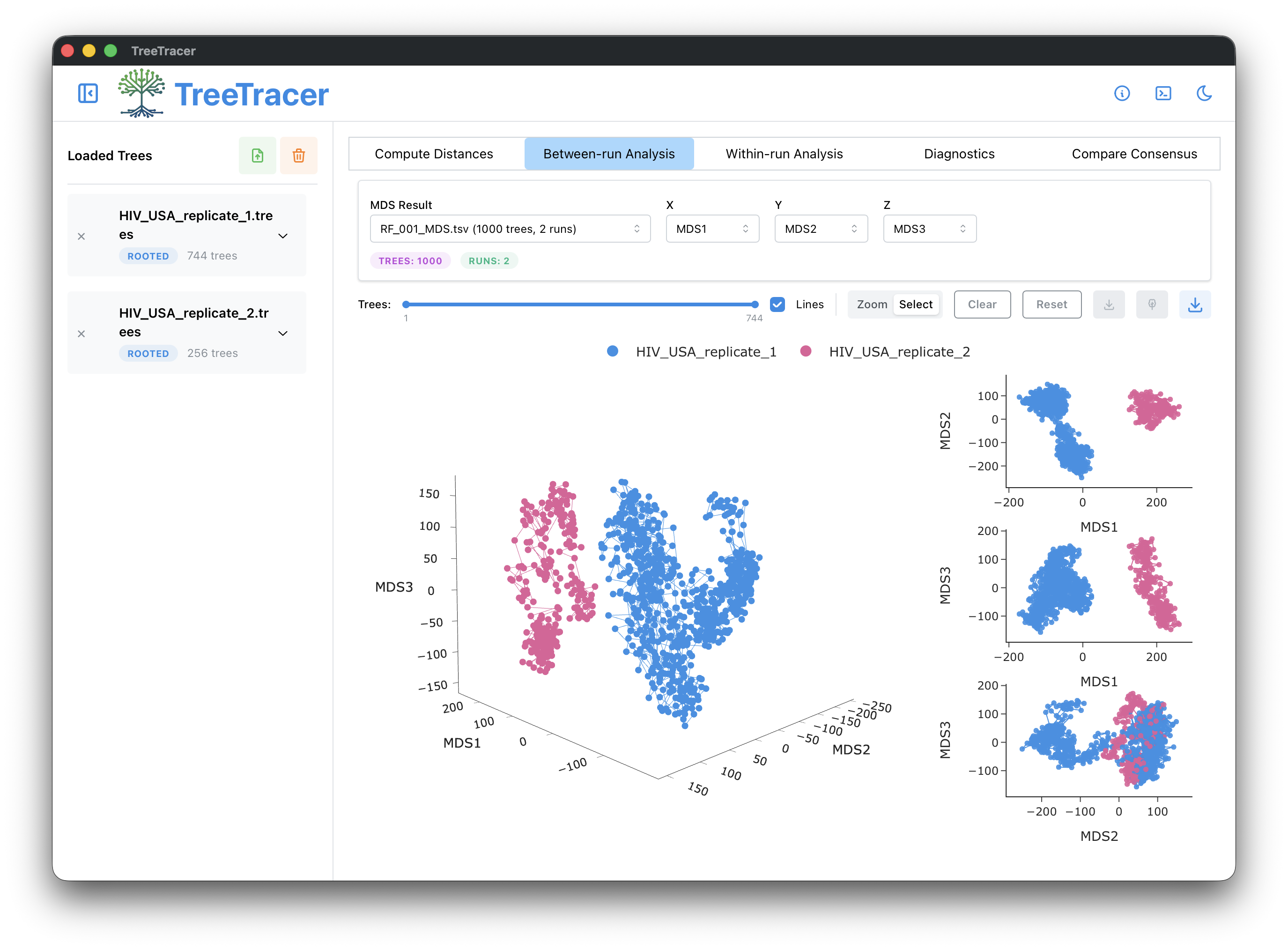
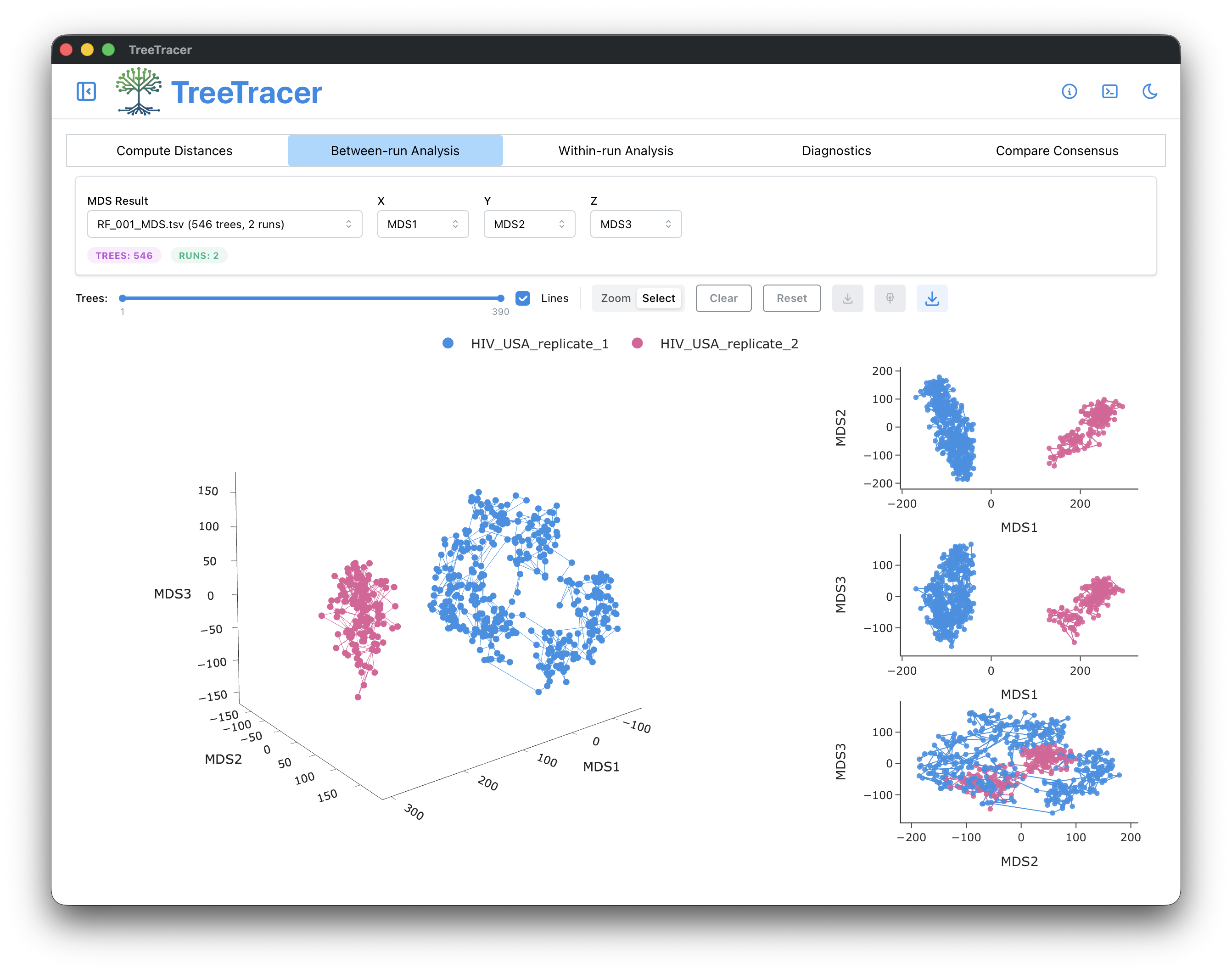
Switching over to the Between-run Analysis panel reveals two distinct point clouds corresponding to our two .trees files in the 3D visualisation but also in two out of the three 2D projections. The point cloud of replicate 1 (in blue) seems to have a tail, warranting further inspection:
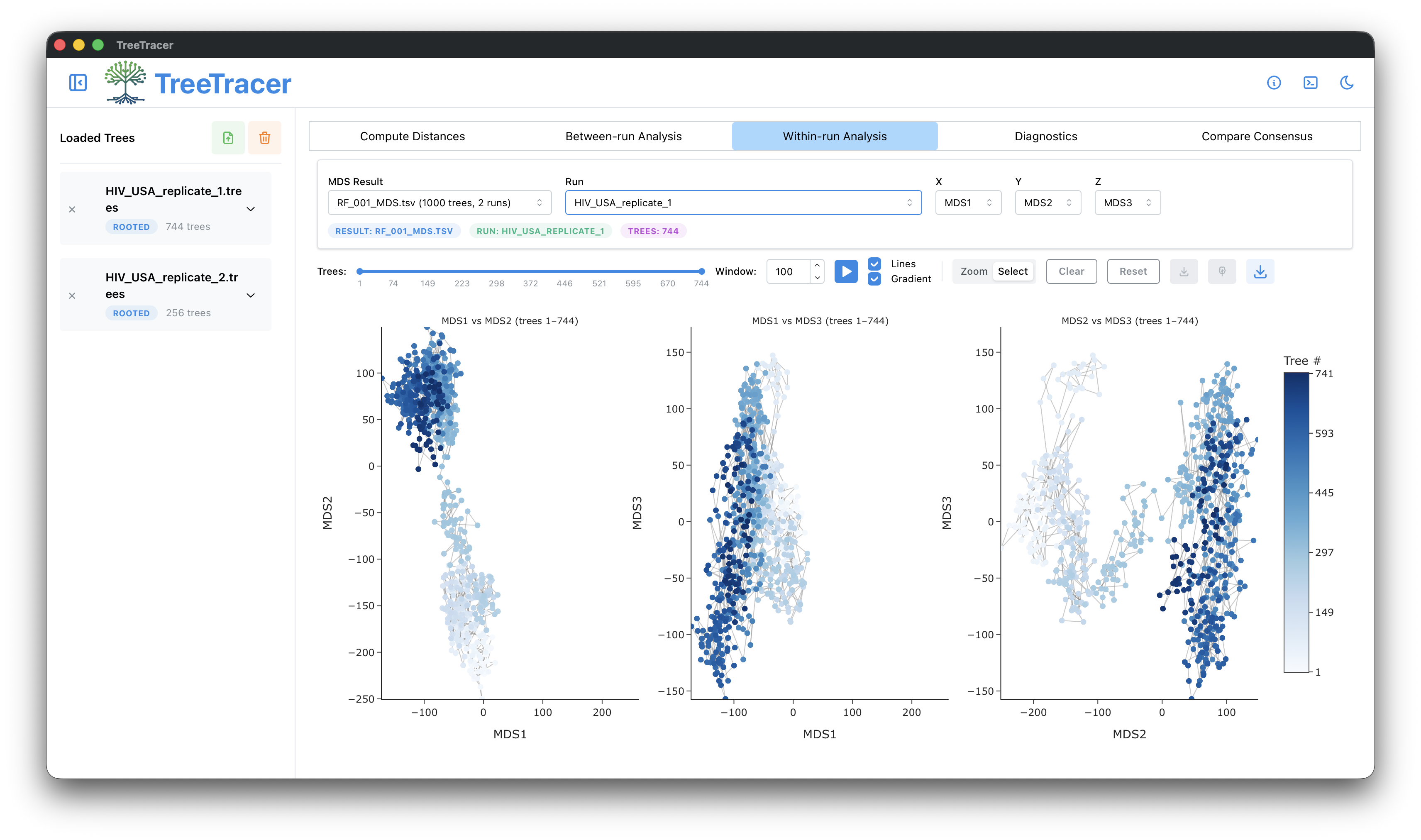
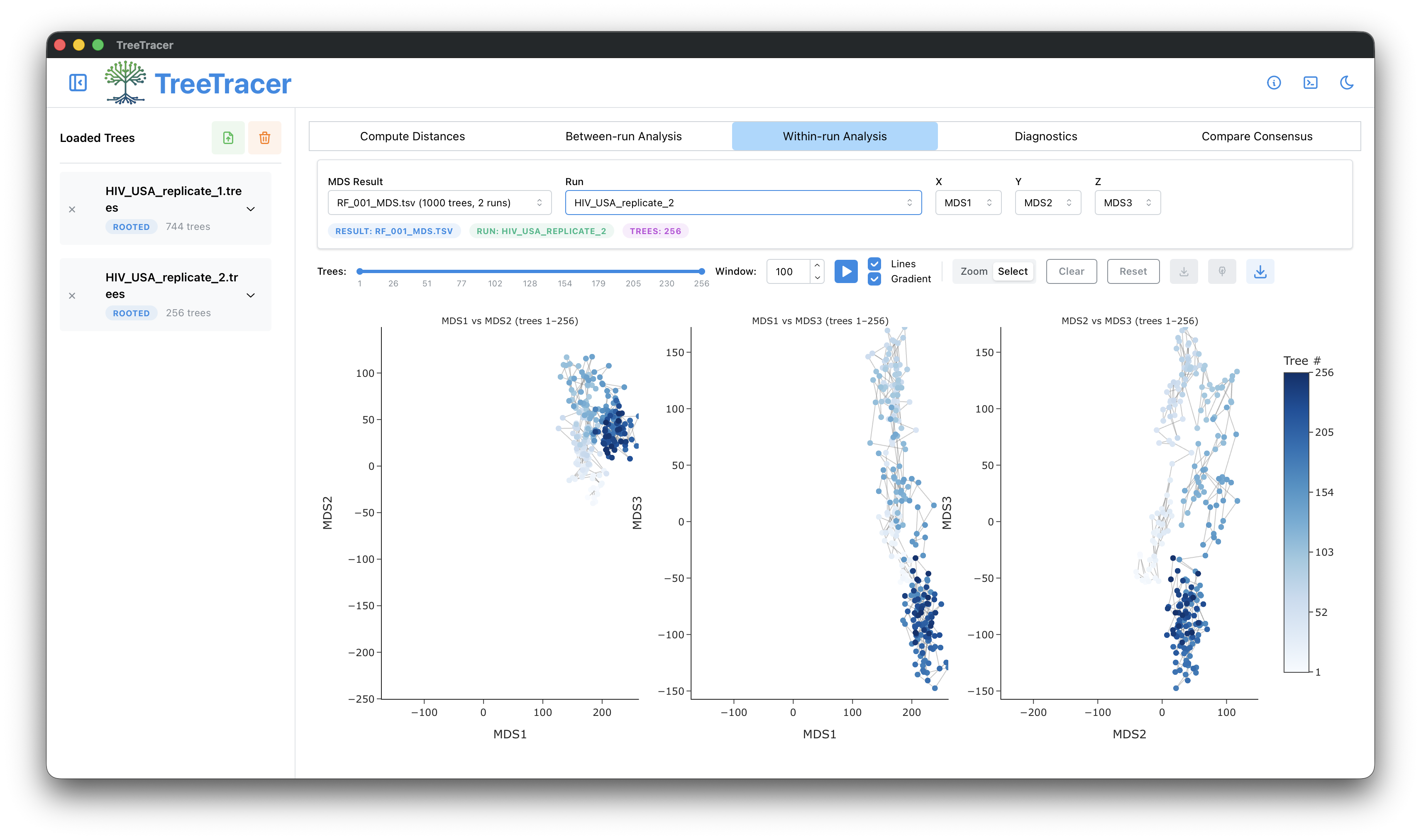
In the Within-run Analysis panel, we immediately see a rather lengthy burn-in present in the sampled trees (the white - very light blue points):
Switching to the second replicate in the same panel, we also see a burn-in still present among the sampled trees:
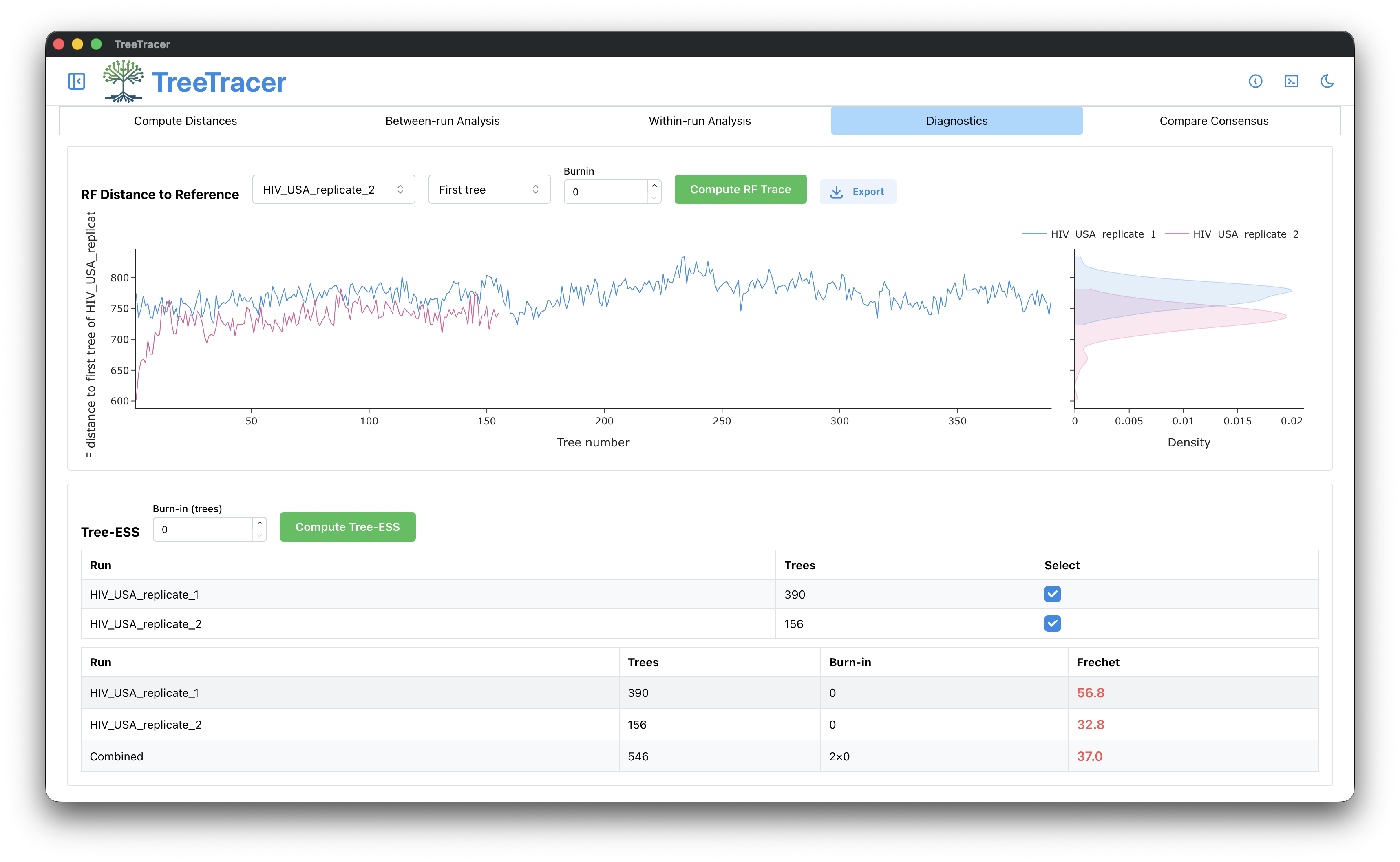
This is confirmed by the Fréchet correlation ESS values (Magee et al., 2024) of the individual replicates and the combined samples. Note how the trace plot of the RF distance to the last sampled tree for the second replicate is showing a downward trend:
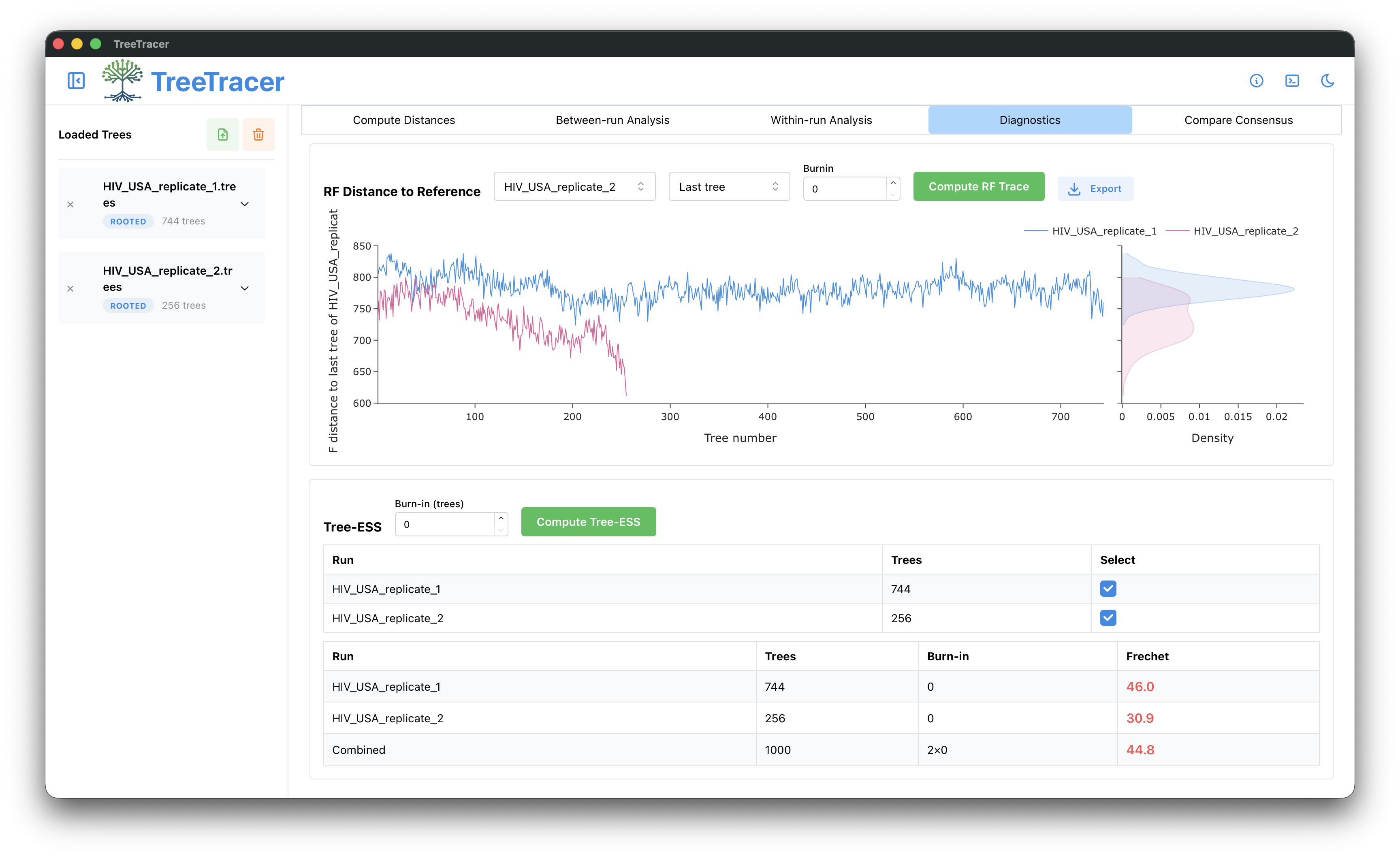
Note that these are the same ESS values as in Brusselmans et al. (2024).
Increasing the burn-in
Given that we saw clear signs of (phylogenetic) burn-in still being present in both .trees files, we can go back to the Compute Distances panel and provide a burn-in for each analysis replicate:
After computing the RF distances and the MDS again, the Between-run Analysis panel looks somewhat better:
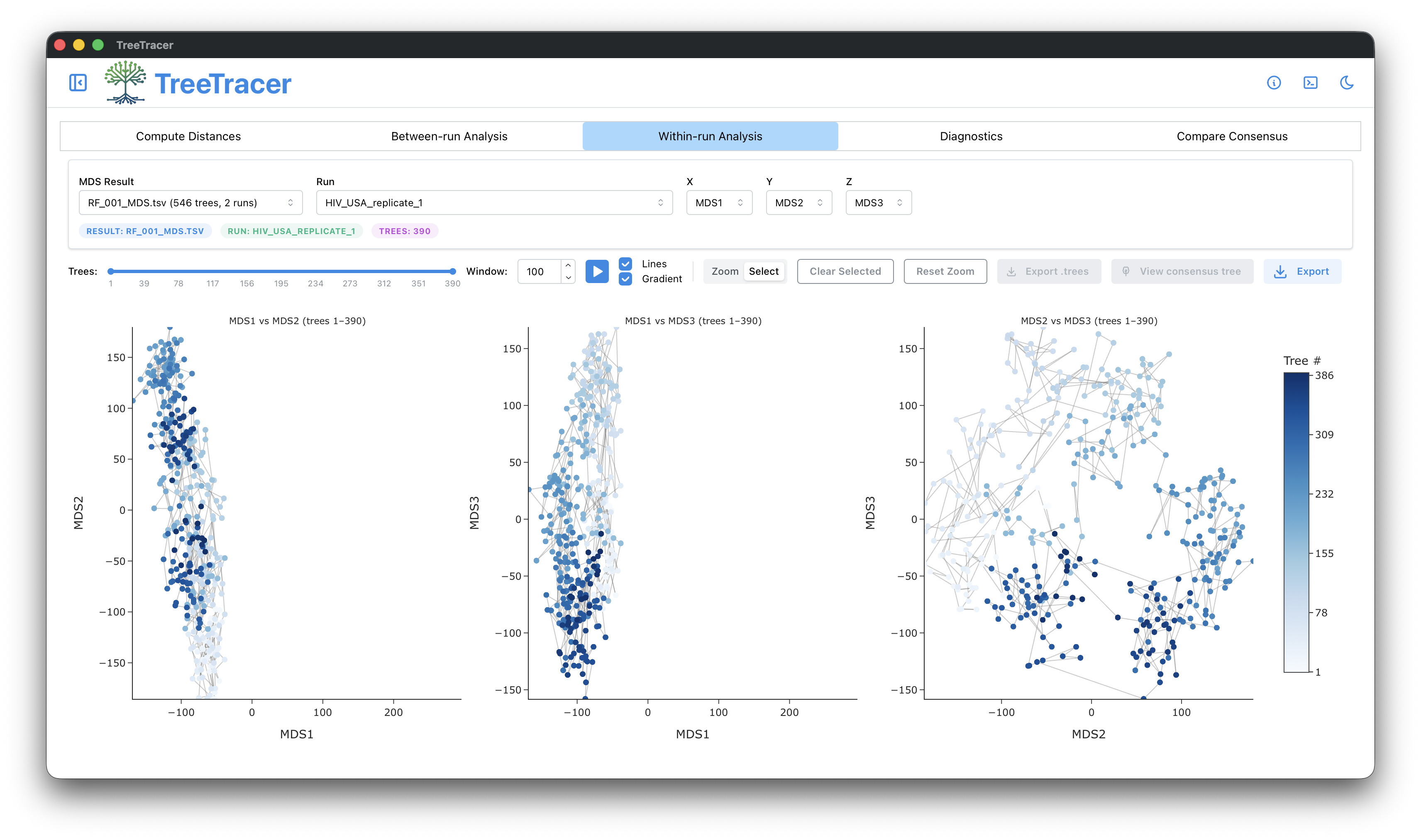
In the Within-run Analysis panel, the first analysis replicate does however still show signs of not all burn-in having been removed:
and the same holds for the second analysis replicate:
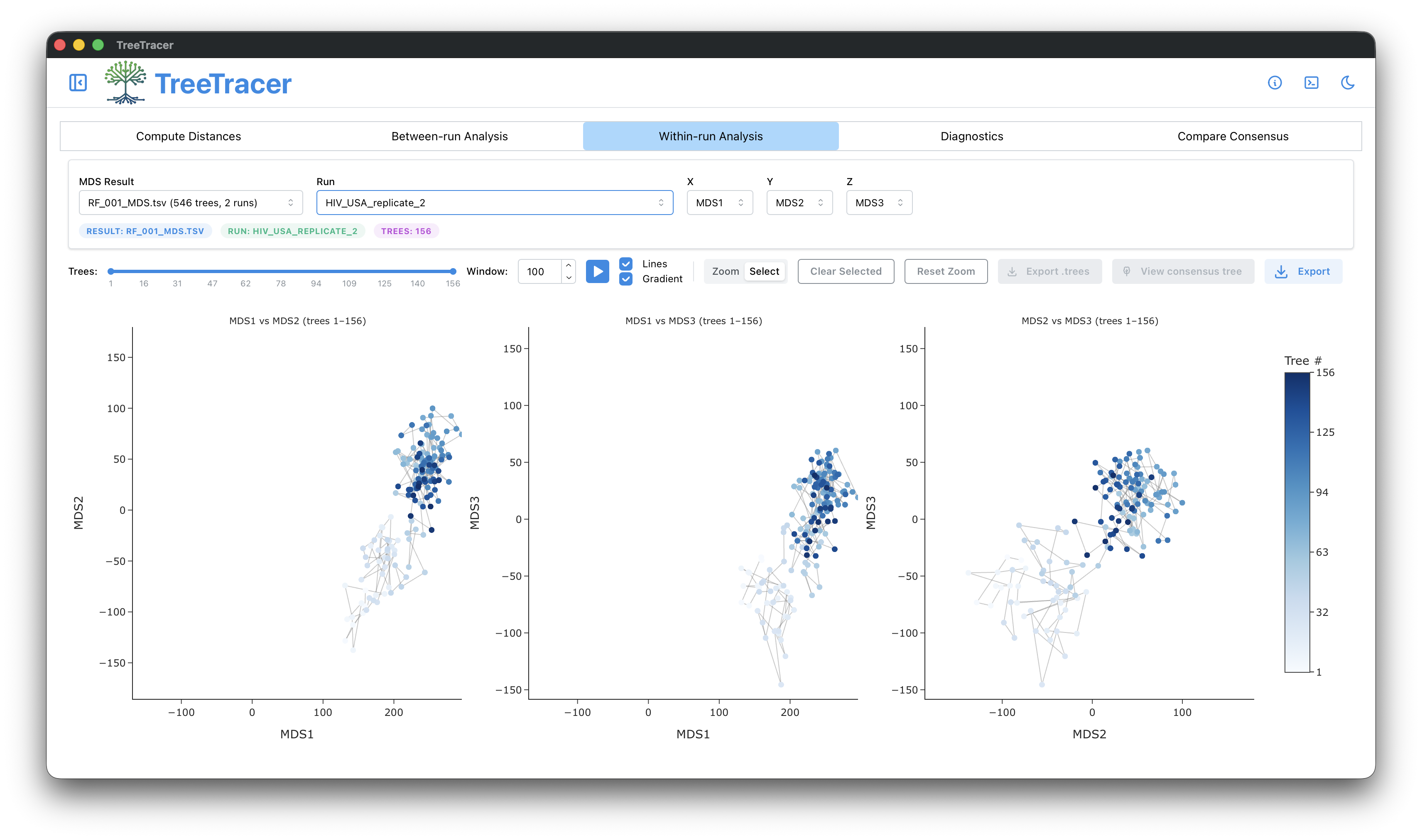
However, increasing the burn-in for both analysis replicates barely increases their Fréchet correlation ESS, and even decreases the Fréchet correlation ESS of the combined sample. This shows (i) that many more samples need to be collected from the posterior and (ii) that the analyses need to be run for longer so as to increase the possibility that they will end up converging to the same posterior, or (iii) a modified analysis with different / additional (tree) transition kernels needs to be run so that different analysis replicates converge to the same posterior.
Conclusion
Many phylogenetic and phylodynamic analyses assess convergence and mixing solely on the sampled continuous parameters and densities. This is clearly insufficient and should be accompanied by inspection of the sampled posterior phylogenies, and ideally a sufficiently high (>500; Magee et al., 2024) Fréchet correlation tree ESS. While there are many different phylogenetic distances metrics than the Robinson-Foulds (RF) metric, it serves at the very least as a good starting point to look for (and potentially remove) rogue taxa in your data set (Gao et al., 2026)
Citing Tracer and TreeTracer
The recommended citation for Tracer is:
Rambaut A, Drummond AJ, Xie D, Baele G and Suchard MA (2018) Posterior summarisation in Bayesian phylogenetics using Tracer 1.7. Systematic Biology. syy032. doi:10.1093/sysbio/syy032
The recommended citation for TreeTracer is:
Hong SL, Brusselmans M, Klaps J, Carvalho LM, Magee AF, Suchard MA, Rambaut A and Baele G (2026) Tree convergence and mixing in Bayesian phylogenetics using TreeTracer. (in preparation).
References
Nylander, J. A. A., Wilgenbusch, J. C., Warren D. L., Swofford, D. L. (2007) AWTY (Are We There Yet?): a system for graphical exploration of MCMC convergence in Bayesian phylogenetics. Bioinformatics 24(4):581-583.
Warren, D. L, Geneva, A. J., Lanfear, R. (2017) RWTY (R We There Yet): an R package for examining convergence of Bayesian phylogenetic analyses. Mol. Biol. Evol. 34(4):1016-1020.
Hong, S. L., Dellicour, S., Vrancken, B., Suchard, M. A., Pyne, M. T., Hillyard, D. R., Lemey, P., Baele, G. (2020) In search of covariates of HIV-1 subtype B spread in the United States - A cautionary tale of large-scale Bayesian phylogeography. Viruses 12(2), 182.
Magee, A., Karcher, M., Matsen IV, F. A., and Minin, V. (2024) How trustworthy is your tree? Bayesian phylogenetic effective sample size through the lens of Monte Carlo error. Bayesian Analysis, 19(2), 565-593.
Brusselmans, M., Carvalho, L. M., Hong, S. L., Gao, J., Matsen IV, F. A., Rambaut, A., Lemey, P., Suchard, M. A., Dudas, G., and Baele, G. (2024) On the importance of assessing topological convergence in Bayesian phylogenetic inference. Virus Evol. 10(1): veae081.
Gao, J., Brusselmans, M., Carvalho, L. M., Suchard, M. A., Baele, G., and Matsen IV, F. A. (2026) Biological causes and impacts of rugged tree landscapes in phylodynamic inference. Proc. Natl. Acad. Sci. USA, 123(2), e2510938123.