
Creating a Figure from a BEAST MCC Tree
This tutorial walks through creating a publication-quality figure from a BEAST MCC (Maximum Clade Credibility) or HIPSTR tree — the kind produced by TreeAnnotator after a BEAST run. It uses the built-in EBOV dataset, which is a timed BEAST MCC tree of 1,610 Ebola virus genomes from the 2014–2016 West Africa epidemic.
What you need
- PearTree web application at https://peartree.live (or the desktop app)
- The built-in EBOV example tree — no download required
- An optional CSV of tip metadata:
data/ebov.csv
What is a BEAST MCC/HIPSTR Tree?
When you run BEAST, it samples a posterior distribution of trees. TreeAnnotator post-processes tens of thousands of sampled trees to produce a single summary tree — either the Maximum Clade Credibility (MCC) tree (BEAST 1+) or a HIPSTR tree (BEAST X 10.5.0+). Both are written as NEXUS files with BEAST metacomments encoding posterior statistics on each node and branch.
The EBOV tree used here carries the following node annotations:
| Annotation | What it represents |
|---|---|
date |
Collection date of the sample (tips only) |
posterior |
Posterior probability of the clade defined by this node (0–1) |
height_mean |
Mean node height (years before the youngest tip) |
height_median |
Median node height |
height_95%_HPD |
95% Highest Posterior Density interval for node height |
height_range |
Full range of sampled node heights |
PearTree reads all of these automatically when you open the file.
Step 1 — Open the Tree
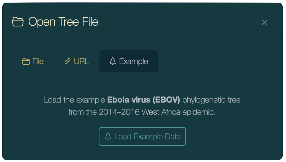
Click the Open button  in the toolbar (or press ⌘O), switch to the Example tab, and click Load Example Data.
Open Tree File dialog, Example tab.
Desktop app: press ⌘O to go directly to a system file browser. Download
data/ebov.treefrom the PearTree GitHub repository and open it, or use File → Open Example from the menu.
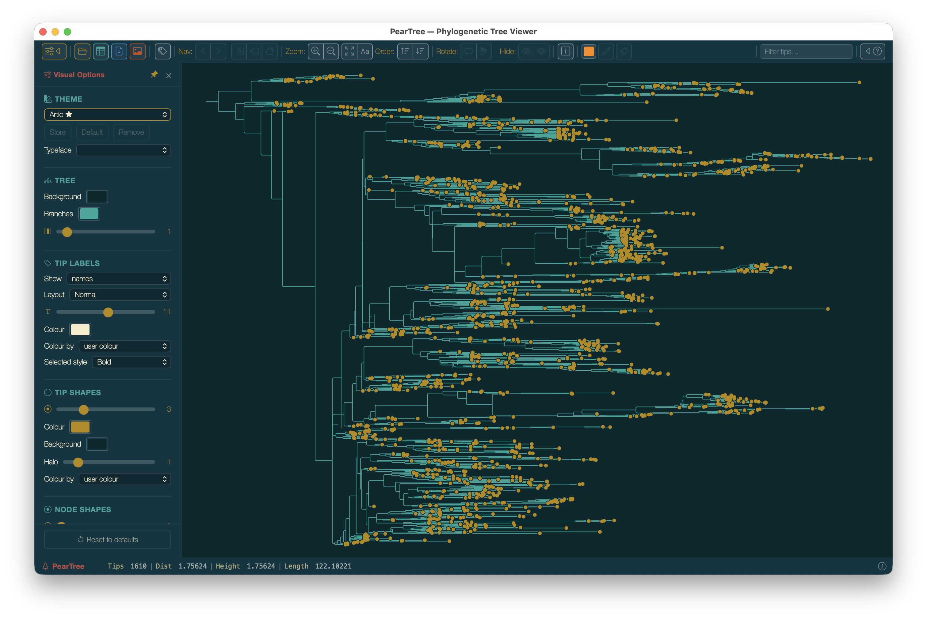
The tree appears on the canvas. Because it is explicitly rooted (BEAST trees always are), the Reroot buttons are disabled.
EBOV MCC tree loaded. At this zoom level tip labels are too small to read — we will use the time axis and visual controls before zooming in.
Step 2 — Order the Branches
MCC trees come out of TreeAnnotator in an arbitrary internal order. Sorting by clade size gives a cleaner ladder layout.
Click Order ↓  (or press ⌘D) to sort clades so the larger clades appear toward the bottom.
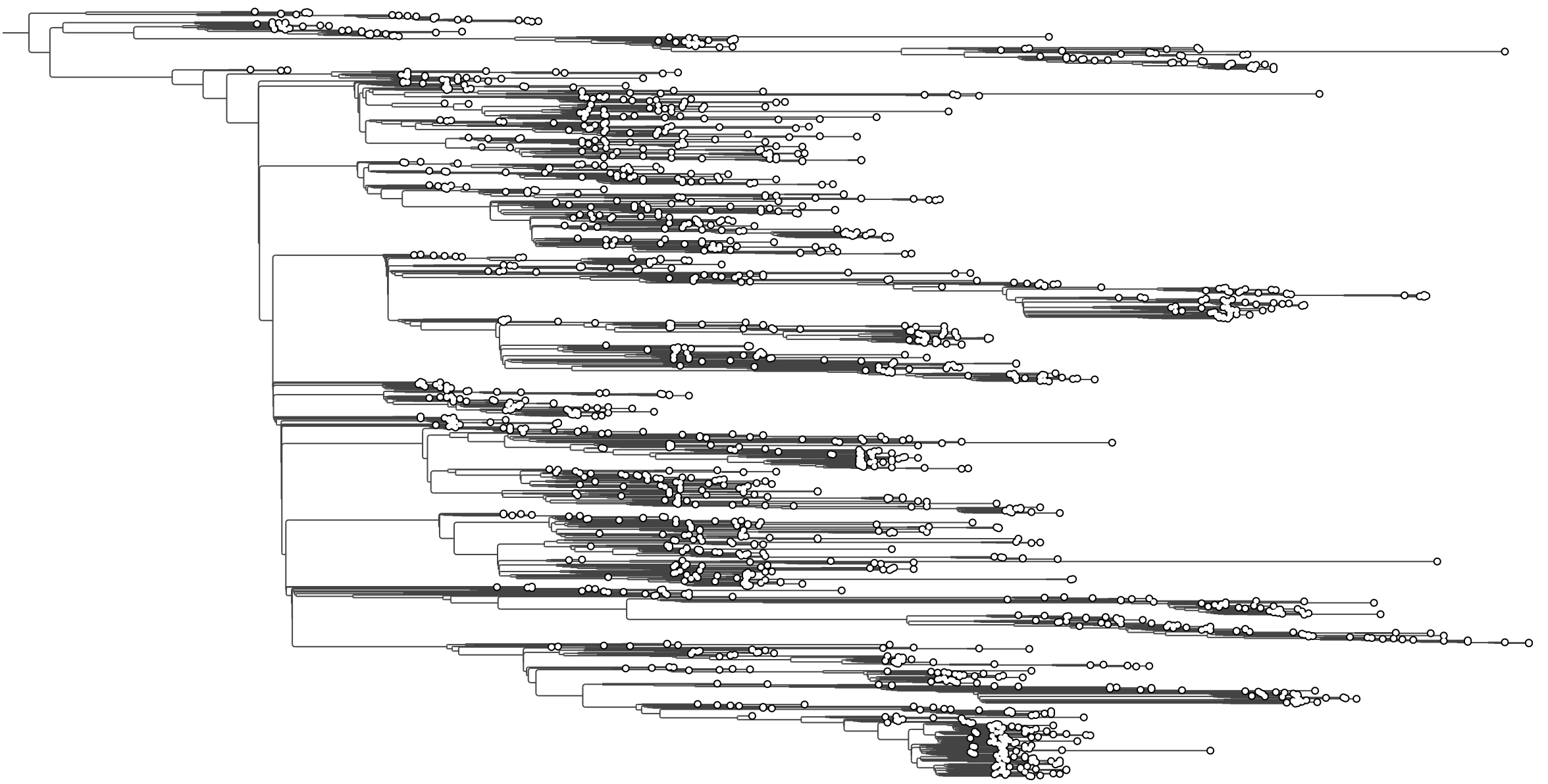
EBOV tree after ordering branches with larger clades toward the bottom.
Step 3 — Add the Time Axis
The EBOV tree is time-calibrated: each branch length is in years. The date annotation on every tip gives the collection date, which allows PearTree to draw a calendar-date axis.
Open the Visual Options palette with the sliders button in the status bar or press Tab.
3a — Calibrate using tip dates
In the Tree section of the palette, set Calibrate to date.
A Format row appears below. The EBOV dates are in ISO format, so leave the format as yyyy-MM-dd.
3b — Enable the time axis
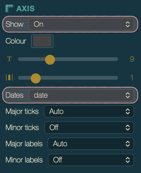
In the Axis section of the palette, set Show to Time.
Suggested tick settings for this dataset:
| Control | Value |
|---|---|
| Major ticks | Years |
| Major labels | Partial |
| Minor ticks | Off |
EBOV tree with a time axis. The epidemic spans 2014–2016.
Step 4 — Show Posterior Support on Nodes
The posterior annotation gives the posterior probability (0–1) that each internal node’s clade exists in the posterior distribution. Values close to 1.0 indicate well-supported clades; values below ~0.5 indicate poorly-supported splits.
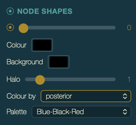
In the Node Shapes section of the palette:
- Set Size to
3(radius in pixels). - Set Colour by to
posterior. - Set Palette to Blue-to-Red (or Blue-Black-Red) — this maps low support to blue and high support to red.
Node Shapes controls with size 3 and Colour by set to
posterior.
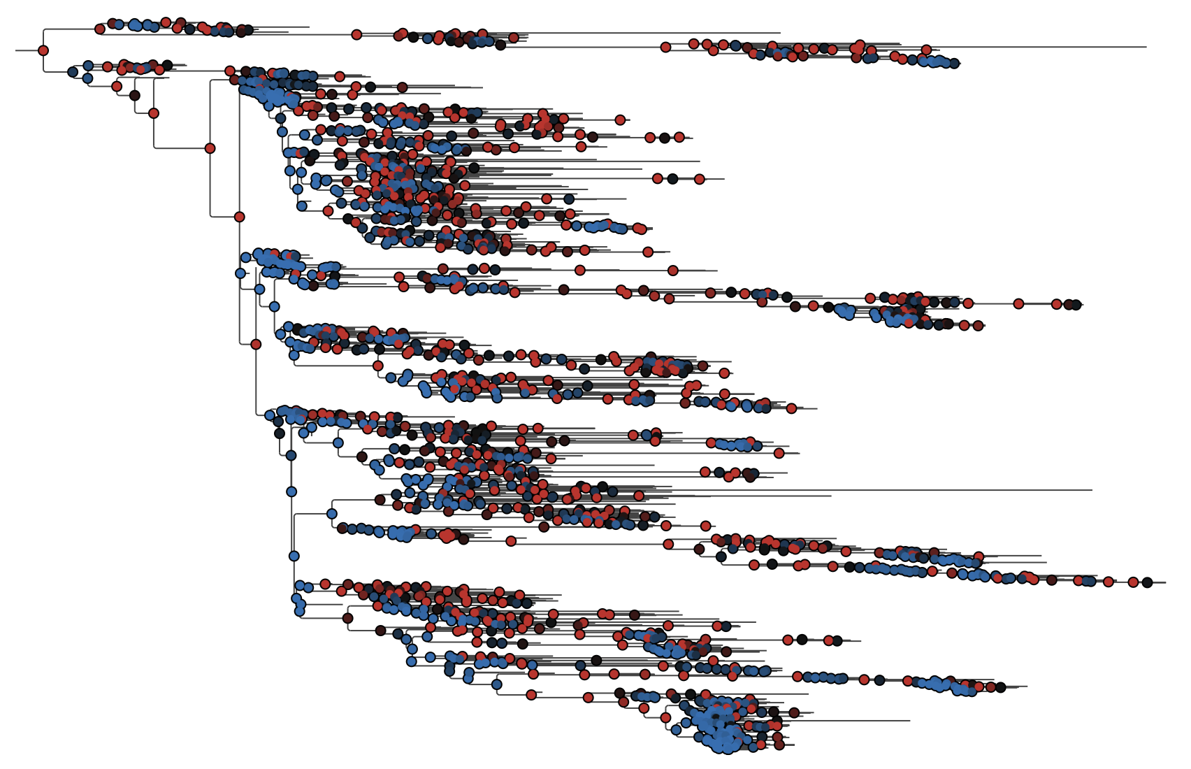
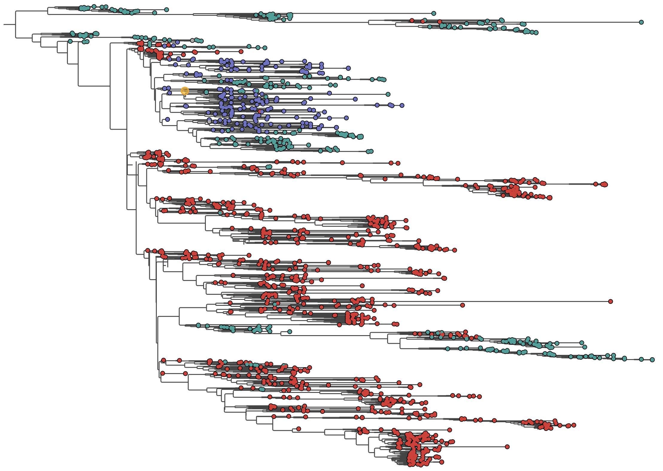
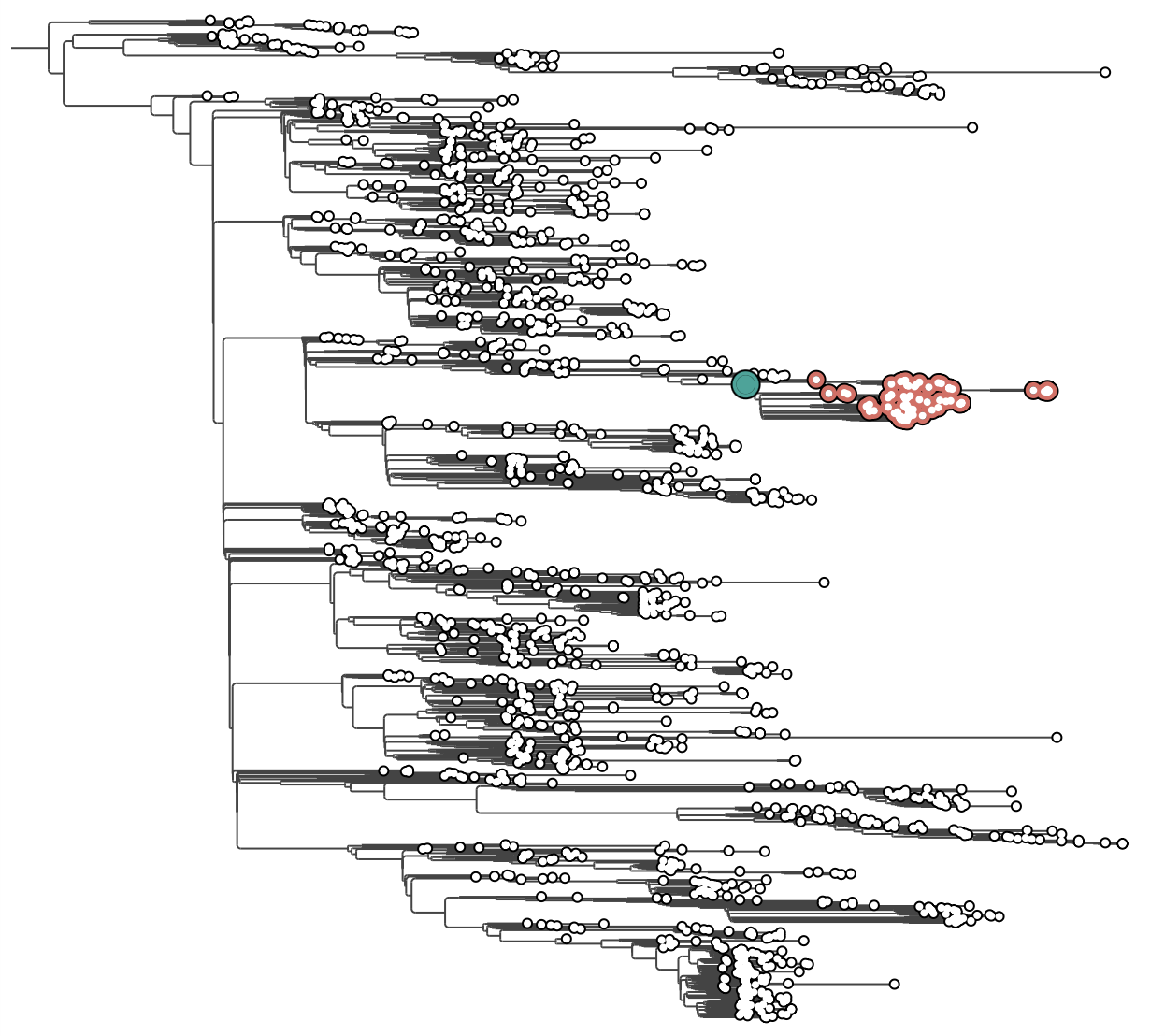
EBOV tree with internal nodes coloured by posterior support. Red = high support (≥0.95), blue = low support (≤0.5).
[!TIP] For publication figures, it is common to show only nodes with
posterior ≥ 0.95— you can achieve this visually by choosing a palette that maps values below your threshold to the background colour, making low-support nodes invisible. Alternatively, use Node Labels to display the exact value as text on specific nodes only.
Step 5 — Show Node Height Uncertainty (HPD Bars)
The height_95%_HPD annotation gives the 95% Highest Posterior Density interval for each node’s height in time. PearTree can draw these as horizontal bars.
In the Node Bars section of the palette (scroll down past Node Labels):
- Set Show to on.
- Set Colour to a light version of the branch colour — a pale grey or semi-transparent colour keeps the bars readable without overwhelming the tree.
- Set Bar height to
2px. - Set Line to
Meanto draw a vertical tick at the posterior mean node height.
Screenshot placeholder — EBOV MCC tree with 95% HPD bars visible at each internal node, coloured pale grey with a mean-position tick.
[!TIP] If the HPD bars make the tree look cluttered, try setting Bar height to 1 px and removing the Line tick. For publication use, HPD bars are most useful in a zoomed-in view of a key clade — use the drill-down function (double-click any internal node) to focus on the clade of interest.
Step 6 — Colour Tips by Sampling Country
The tree labels are in the format EBOV|sample-id|accession|collection-date. To add richer metadata — sampling country, location, and other fields — import the companion CSV file.
6a — Import the annotation file
Click the annotation-import button  in the toolbar (or press ⌘⇧A).
Import Annotations dialog.
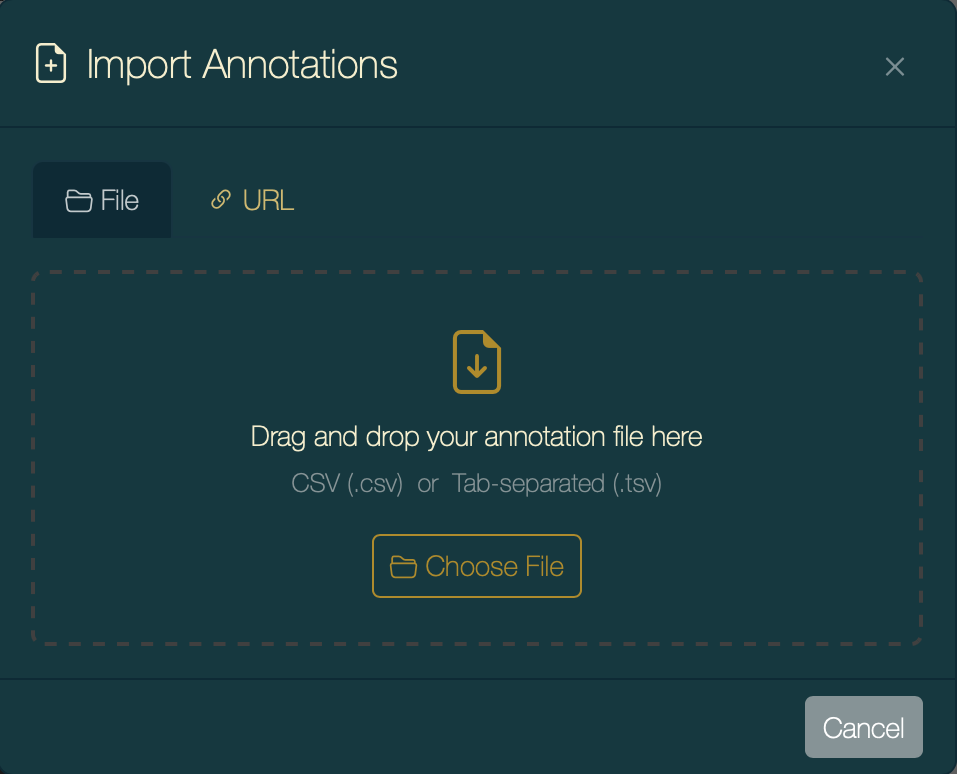
Switch to the URL tab and paste:
https://artic-network.github.io/peartree/docs/data/ebov.csv
Then click Load from URL.
Desktop app: switch to the File tab, download
data/ebov.csvfrom the PearTree GitHub repository and open it.
6b — Configure the match
In the match configuration step, set Match on field to 2 — the second pipe-delimited segment of each tip label is the sample ID, which matches the lab-id column in the CSV.
Import configuration: match field 2 (sample ID) to the
lab-idcolumn.
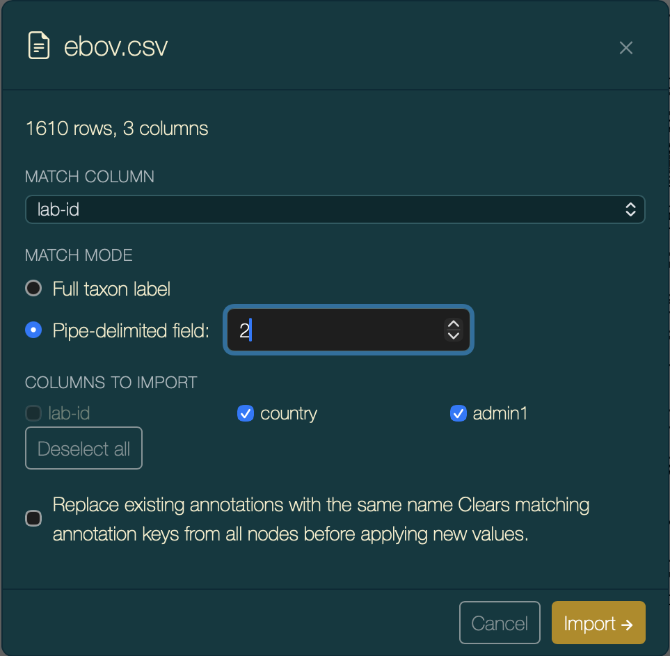
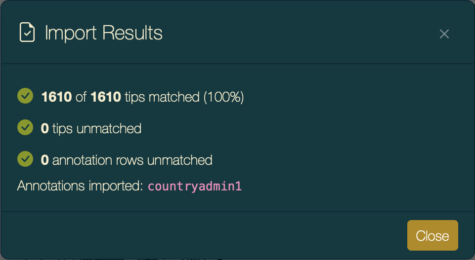
Click Import. The summary confirms all 1,610 tips matched.
Import summary showing all tips matched.
6c — Colour tips by country
In the Tip Shapes section of the palette:
- Set Colour by to
country. - Choose a categorical palette — Tableau 10 or Set1 work well.
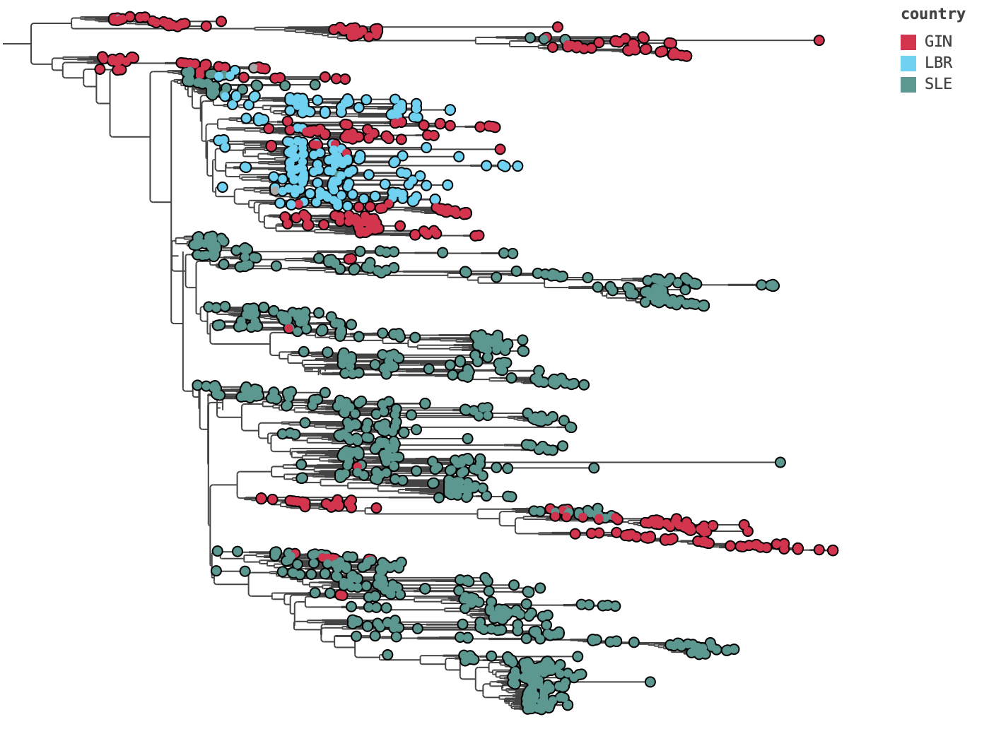
EBOV tips coloured by sampling country. Mixing of countries across the tree reflects the regional connectivity of the epidemic.
Step 7 — Add a Country Legend
In the Legend section of the palette:
- Set Annotation to
country. - Set Font size to
10. - Adjust Height % so the legend occupies approximately 40–60% of the canvas height.
EBOV tree with country tip colours and a colour legend docked to the right.
Step 8 — Zoom In and Inspect
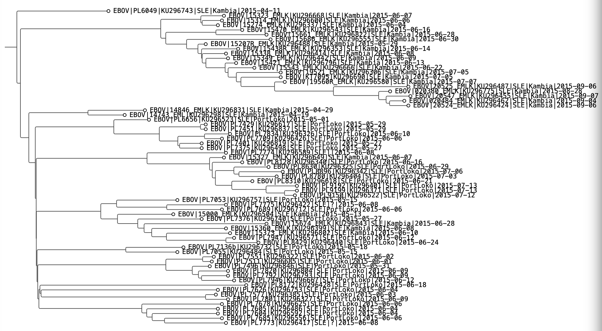
Use Fit Labels ( or ⌘⇧0) to zoom to label-readable spacing.
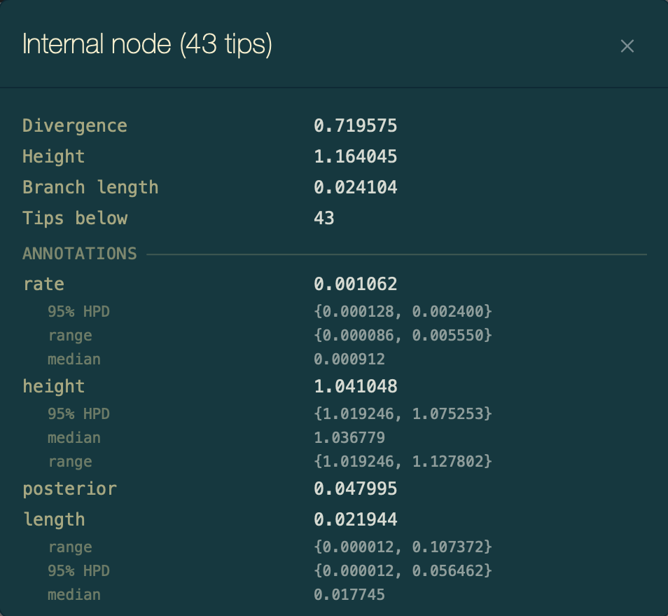
Click any tip to select it and show its values in the status bar at the bottom. Press ⌘I or click the info button to open the Node Info dialog, which lists all annotations for that tip including the imported metadata.
Node Info dialog for a selected EBOV tip, showing all annotations including the imported country and location fields.
To inspect a specific clade in detail, double-click any internal node to drill down into it:
A subclade before drilling down (top) and after (bottom), with HPD bars and posterior colours visible.
Press ⌘\ to return to the full tree view.
Step 9 — Export the Figure
SVG (recommended for publications)
Press ⌘⇧E or click the export graphic button. Choose:
| Option | Value |
|---|---|
| Format | SVG |
| View | Full tree (to include the entire tree, not just the visible viewport) |
| Transparent background | Tick, if you plan to composite onto a coloured page |
Export Graphic dialog with SVG and Full tree selected.
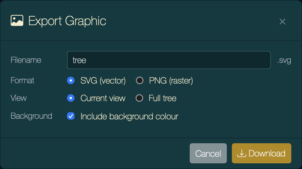
The SVG contains fully vector branches, labels, node circles, HPD bars, legend, and time axis — ideal for editing in Illustrator or Inkscape, or embedding directly in a manuscript PDF.
PNG (presentations and web)
Choose PNG if you need a raster image. PearTree exports at 2× screen resolution.
Embed settings for collaboration
If you want to share the figure configuration with a colleague or preserve it for revision, export the tree as NEXUS with Embed settings ticked (press ⌘S):
Export Tree dialog with Embed settings ticked.
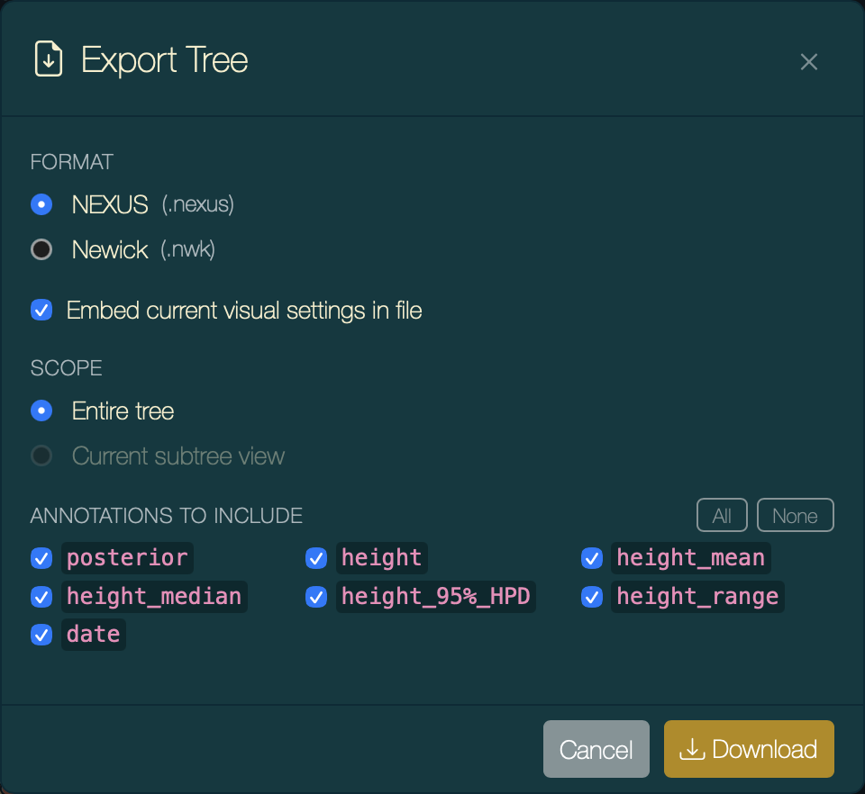
Opening the resulting .nexus file in any copy of PearTree automatically restores tip colours, node shapes, HPD bars, time axis, legend, and theme — no manual reconfiguration required.
Summary
| Step | What you did | Key annotations used |
|---|---|---|
| 1 | Opened the BEAST MCC tree | (tree file) |
| 2 | Ordered branches by clade size | — |
| 3 | Added a time-calibrated axis | date |
| 4 | Coloured internal nodes by support | posterior |
| 5 | Added 95% HPD bars | height_95%_HPD, height_mean |
| 6 | Imported metadata and coloured tips | country (from CSV) |
| 7 | Added a legend | country |
| 8 | Zoomed in and inspected nodes | all annotations |
| 9 | Exported as SVG / embedded settings | — |
Going Further
- Sharing a live link — export the tree as NEXUS with embedded settings, host the file publicly (e.g. on GitHub), and share the URL:
https://peartree.live/?treeUrl=<raw-file-URL>. Recipients see the fully-configured figure immediately in their browser.