Introduction
The first step will be to convert an alignment file in fasta format into a BEAST XML input file. This is done using the program BEAUti (this stands for Bayesian Evolutionary Analysis Utility). This is a user-friendly program for setting the evolutionary model and options for the MCMC analysis. The second step is to actually run BEAST using the input file that contains the data, model and settings. The final step is to explore the output of BEAST in order to diagnose problems and to summarize the results.
To undertake this tutorial, you will need to download three software packages in a format that is compatible with your computer system (all three are available for Mac OS X, Windows and Linux/UNIX operating systems):




EXERCISE 1: discrete ancestral reconstruction
Running BEAUti

Loading the sequence data file
The input file for this tutorial, EBOV_DRC_18-20.fas, can be downloaded from here. This fasta formatted file contains an alignment of 836 EBOV genomes encompassing 18750 bp.
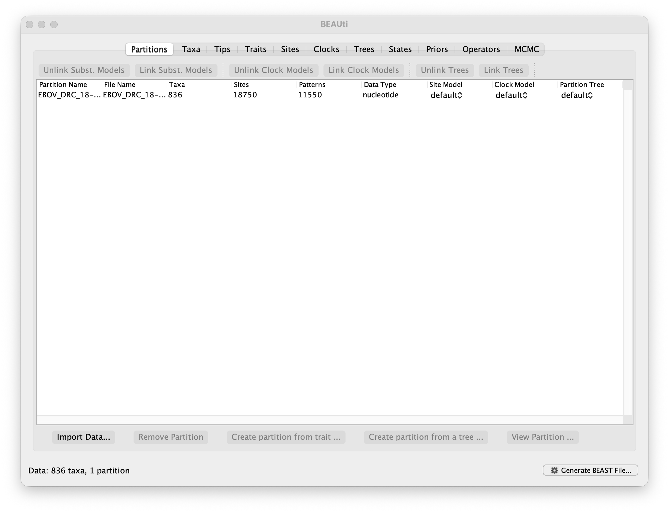
To load the alignment, simply select the Import Data... option from the File menu. Select the EBOV_DRC_18-20.fas file. Alternatively, you can drag and drop the alignment file in the window under the Partitions menu.
Once loaded, the sequence data will be listed under Partitions as shown in the figure:
Specifying the sampling date information
By default all the taxa are assumed to have a date of zero (i.e. the sequences are assumed to be sampled at the same time). However, the EBOV sequences have been sampled over about a year. To set the sampling dates switch to the Tips panel using the tabs at the top of the window.
Select the box labelled Use tip dates. The EBOV sequences have their date of sampling encoded in their labels so use the Parse Dates button at the top of the Tips panel. Clicking this will make a dialog box appear:
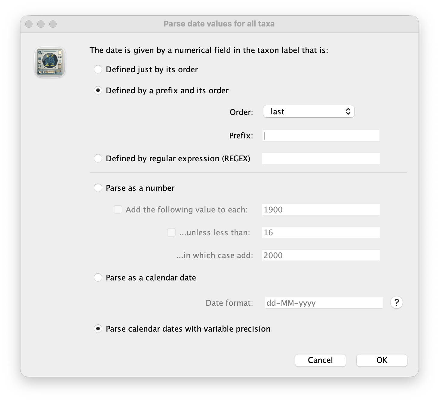
This operation attempts to guess what the dates are from information contained within the taxon names. It works by trying to find a numerical field within each name. If the taxon names contain more than one numerical field then you can specify how to find the one that corresponds to the date of sampling. See this page for details about the various options for setting dates in this panel. For the EBOV sequences you can specify Defined by a prefix its order, Order: last, Prefix: | and Parse calendar dates with variable precision. The latter is needed because for 4 genomes, only the month of sampling is known. Press OK. A window should appear to indicate that some dates have less precision than others, offering to switch on Sampling uniformly from precision. Press Yes. The dates (Date) and their uncertainty (Uncertainty) will appear in the appropriate columns of the main window, and the Tip date sampling option at the bottom left of the Tips panel will be set to Sampling uniformly from uncertainty.
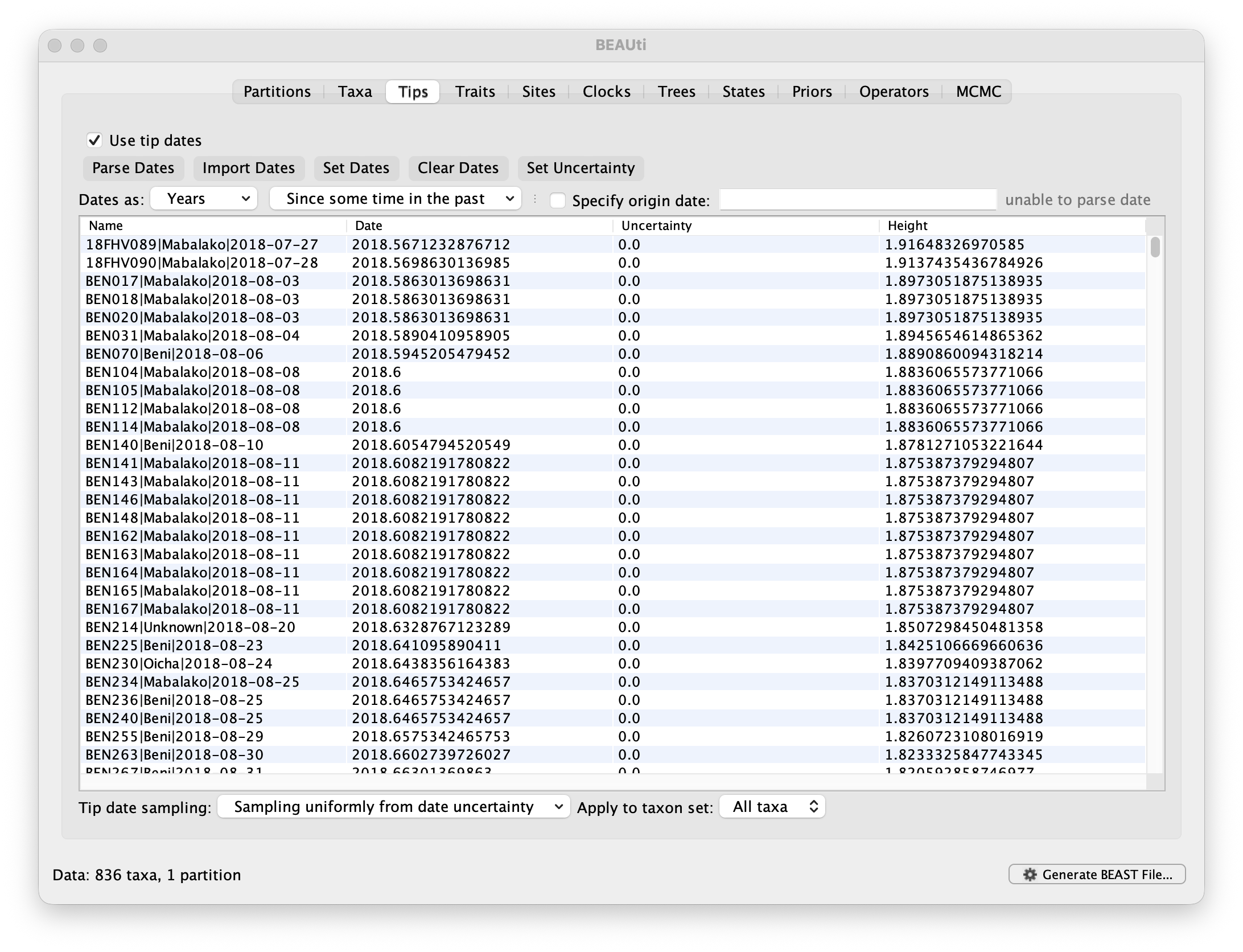
You can now check these dates (as fractional years) and edit them manually if that would be needed. At the top of the window you can set the units that the dates are given in (years, months, days) and whether they are specified relative to a point in the past (as is the case for years such as 2005) or backwards in time from the present (as in the case of radiocarbon ages).
The Height column lists the ages of the tips relative to time 0 (in our case, the most recent sampling date: 2019-08-03 or 2019.5863013698631). You can change the ‘time 0’ date by clicking the Specify origin date: option and specifying it in the respective window.
Specifying the trait information
The next thing to do is to click on the Traits tab at the top of the main window. A trait can be any characteristic that is inherent to the specific taxon, for example, geographical location or host species. This step will assign a geographical location to each taxa based on the trait specification for each sequence in the taxa_HZ.txt file, which can be downloaded from here. To associate the sequences with the traits, we need to add a new trait under the Traits tab (click Add trait). This will open a new window to Create or Import Trait(s):
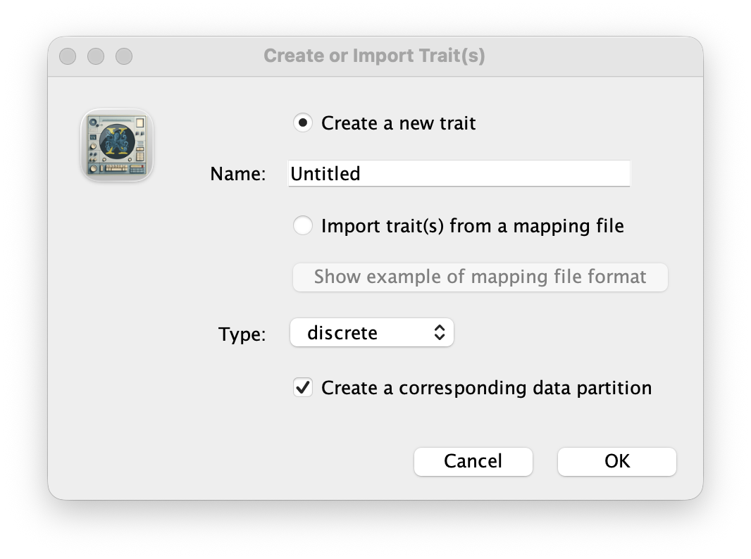
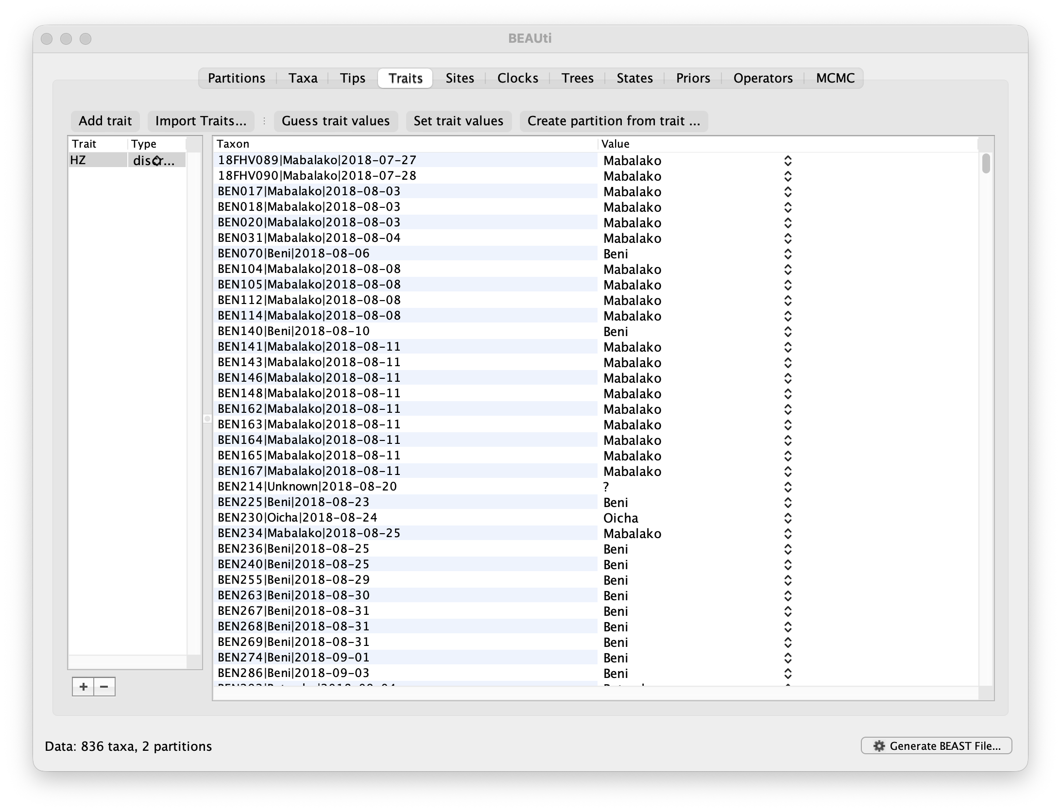
Select Import trait(s) from a mapping file (the format of such a file can be shown). Browse to and load the taxa_HZ.txt tab-delimited file. A window will appear asking you whether you want to create a traits partition: Press Yes. In the next window, set Name trait partition: to HZ(for health zone).
The HZ trait should now appear in the left window and clicking on it shows the health zone locations associated with the taxa.
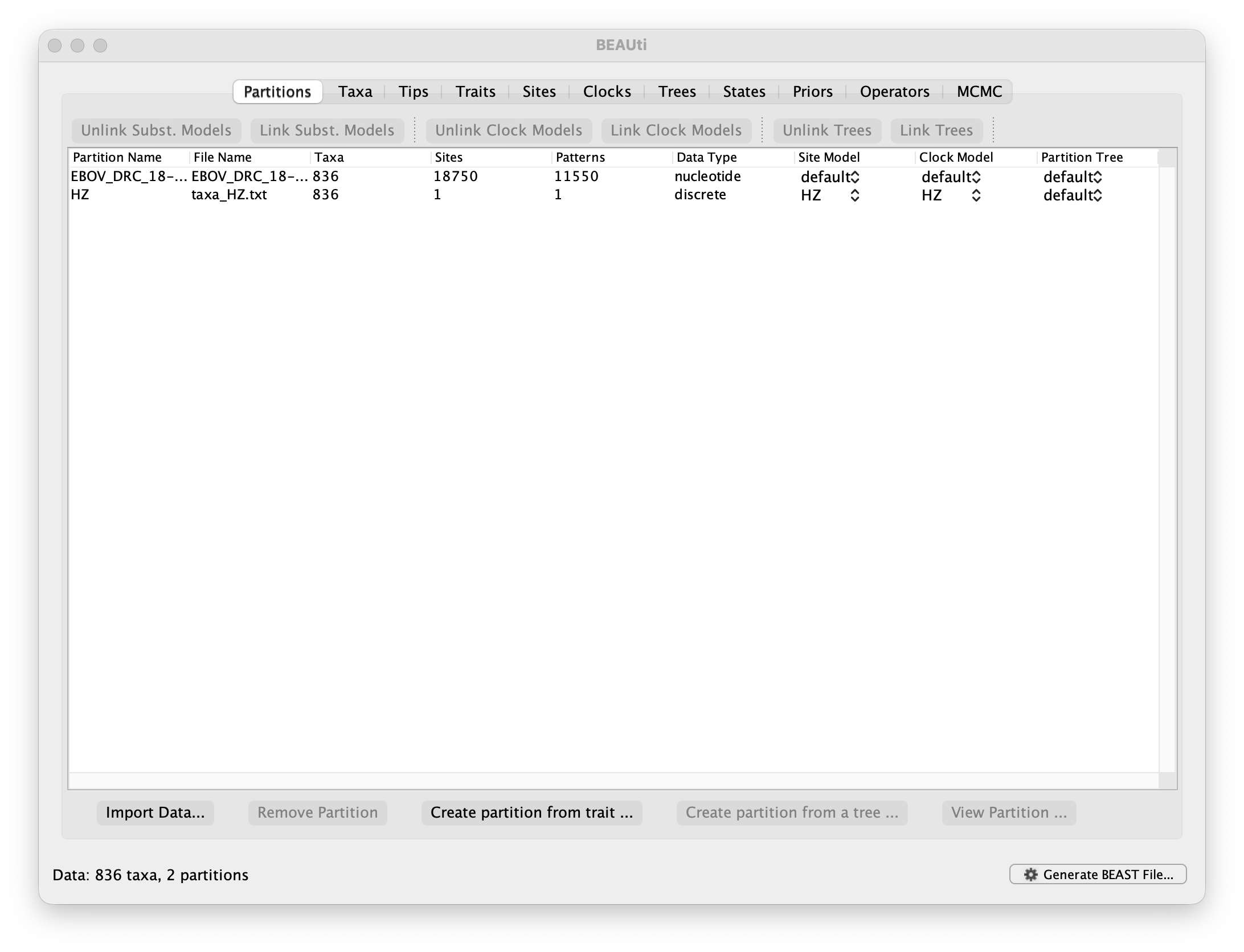
The new partition will also be shown under the Partitions tab, resulting in two partitions in the Partitions tab:
Setting the sequence and trait evolutionary models
The next thing to do is to click on the Sites tab at the top of the main window. This will reveal the evolutionary model settings for BEAST. For the nucleotide model in this tutorial, we specify the GTR substitution model, we set base frequencies to Empirical, and use Gamma-distributed rate variation among sites (with 4 discrete categories, the Gamma (equal weights) option):
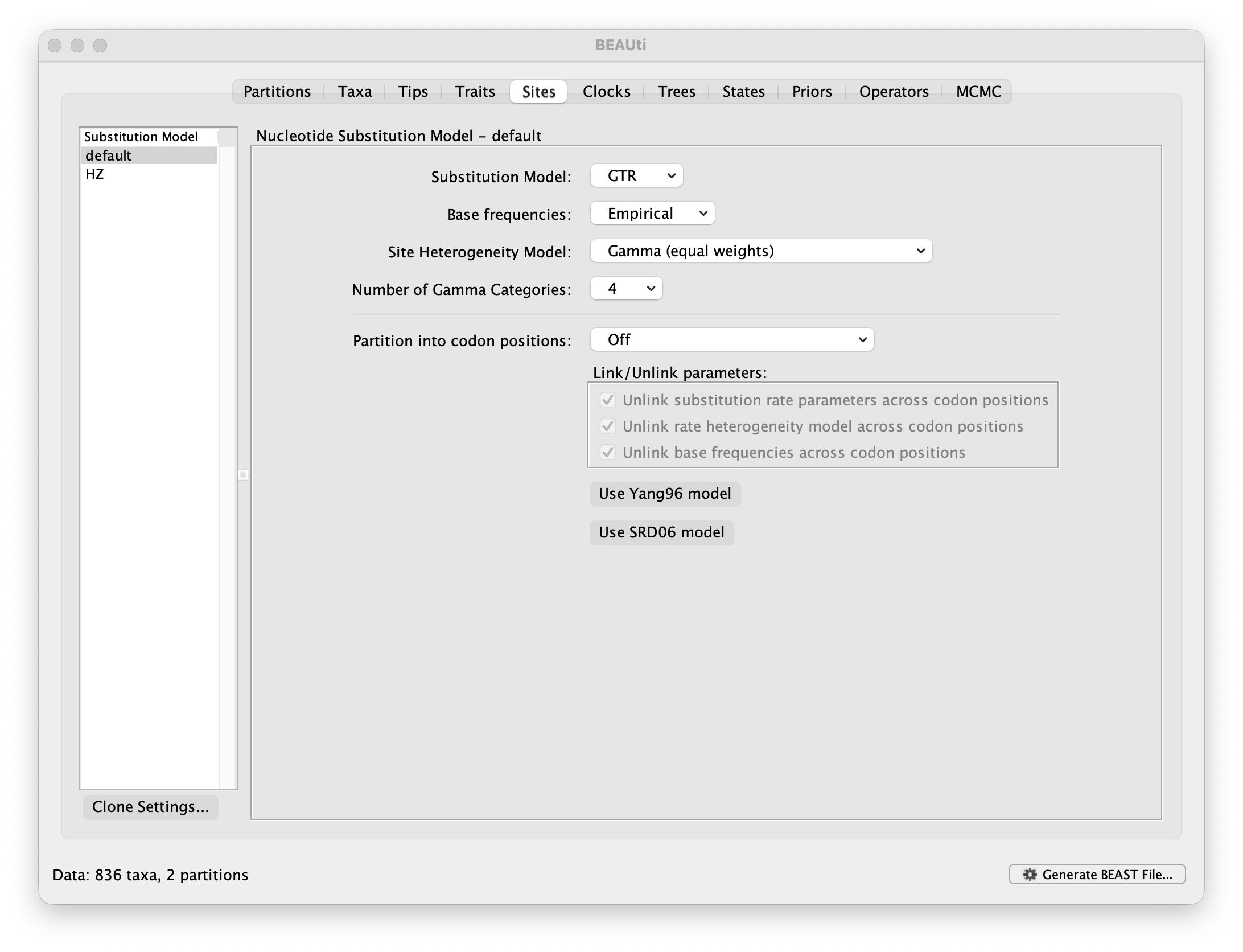
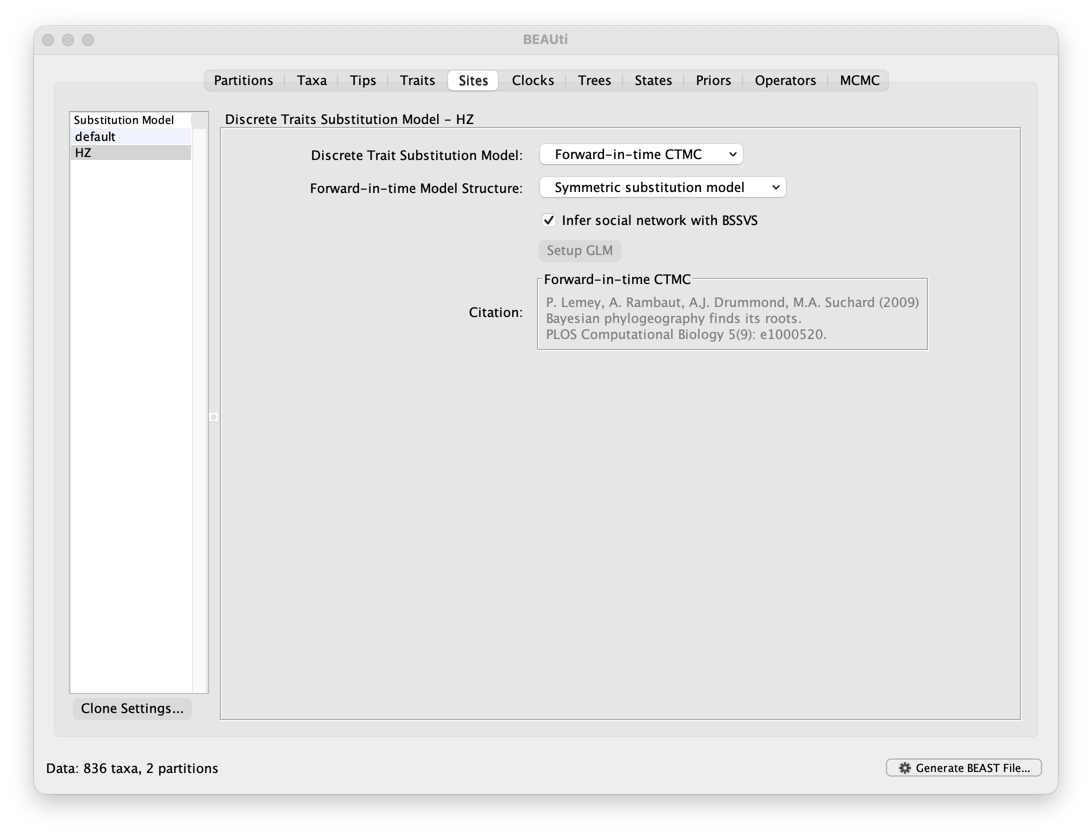
Next, click on ‘HZ’ in the Substitution model window and keep the Forward-in-time CTMC model as Discrete Trait Substitution Model and the Symmetric substitution model as Forward-in-time Model Structure, but select the option to perform BSSVS (Infer social network with BSSVS). The symmetric substitution model specifies a discrete state ancestral reconstruction using a standard continuous-time Markov chain (CTMC), in which the transition rates between locations are reversible. The alternative Asymmetric substitution model specifies a discrete state ancestral reconstruction using a nonreversible CTMC. Selecting the BSSVS option enables the Bayesian Stochastic Search Variable Selection procedure. This procedure will attempt to limit the number of rates (at least K-1, where K is the number of states) to only those that adequately explain the phylogenetic diffusion process.
Setting the ‘molecular clock’ model
The ‘Molecular Clock Model’ options in the Clocks panel allows us to choose between a strict and a relaxed (uncorrelated lognormal or uncorrelated exponential) clock. For the nucleotide data (default), we will perform our run using the Uncorrelated relaxed clock model with the default Lognormal distribution as Relaxed Distribution:
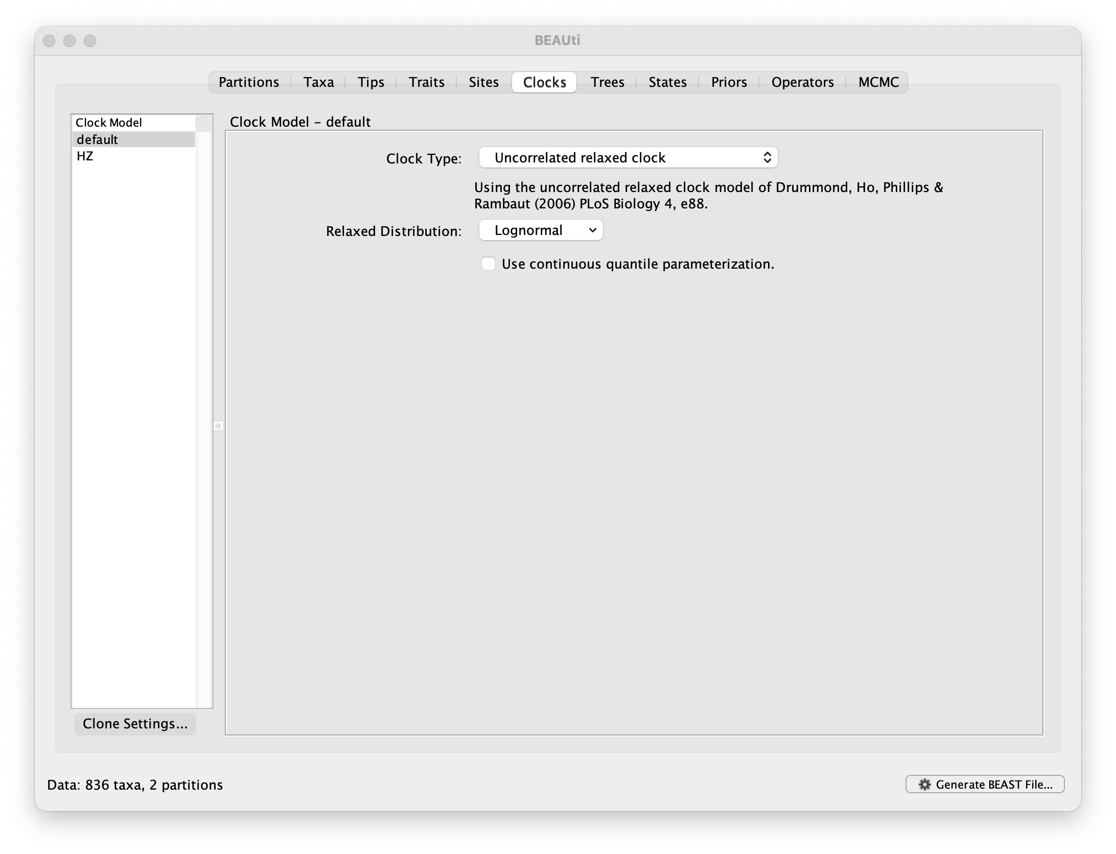
We can keep the default settings for overall rate scalar on the geographic HZ transition processes.
Now move on to the Trees panel.
Setting the tree prior
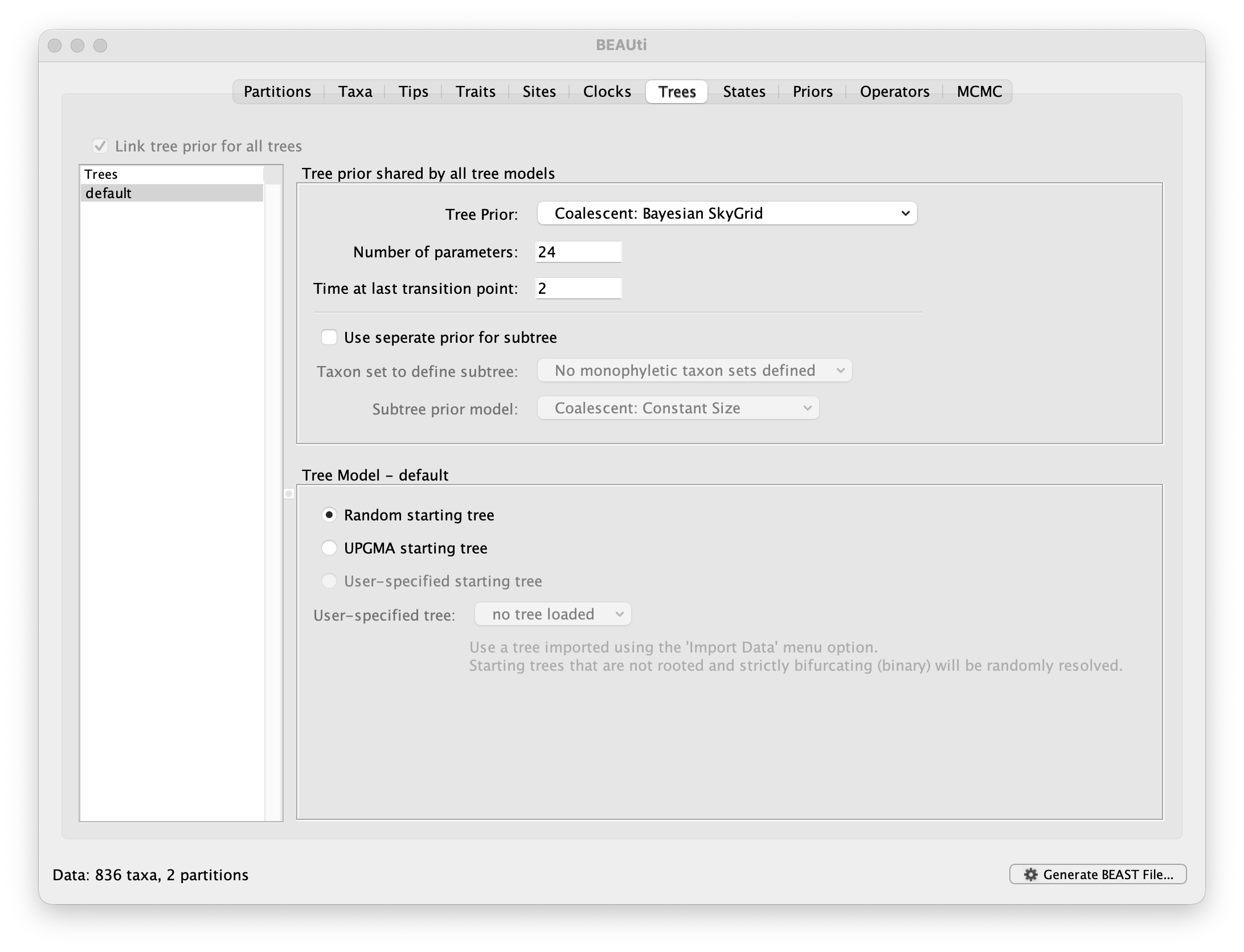
This panel contains settings about the tree. Firstly the starting tree is specified to be a Random starting tree. The other main setting here is to specify the Tree prior which describes how the population size is expected to change over time according to a coalescent model. The default tree prior is set to a constant size coalescent prior. In this tutorial, we will set the Tree Prior: to Coalescent: Bayesian SkyGrid with 24 population sizes (Number of parameters: 24) for a period of two years, so with Time at last transition point: 2.
The ancestral states settings
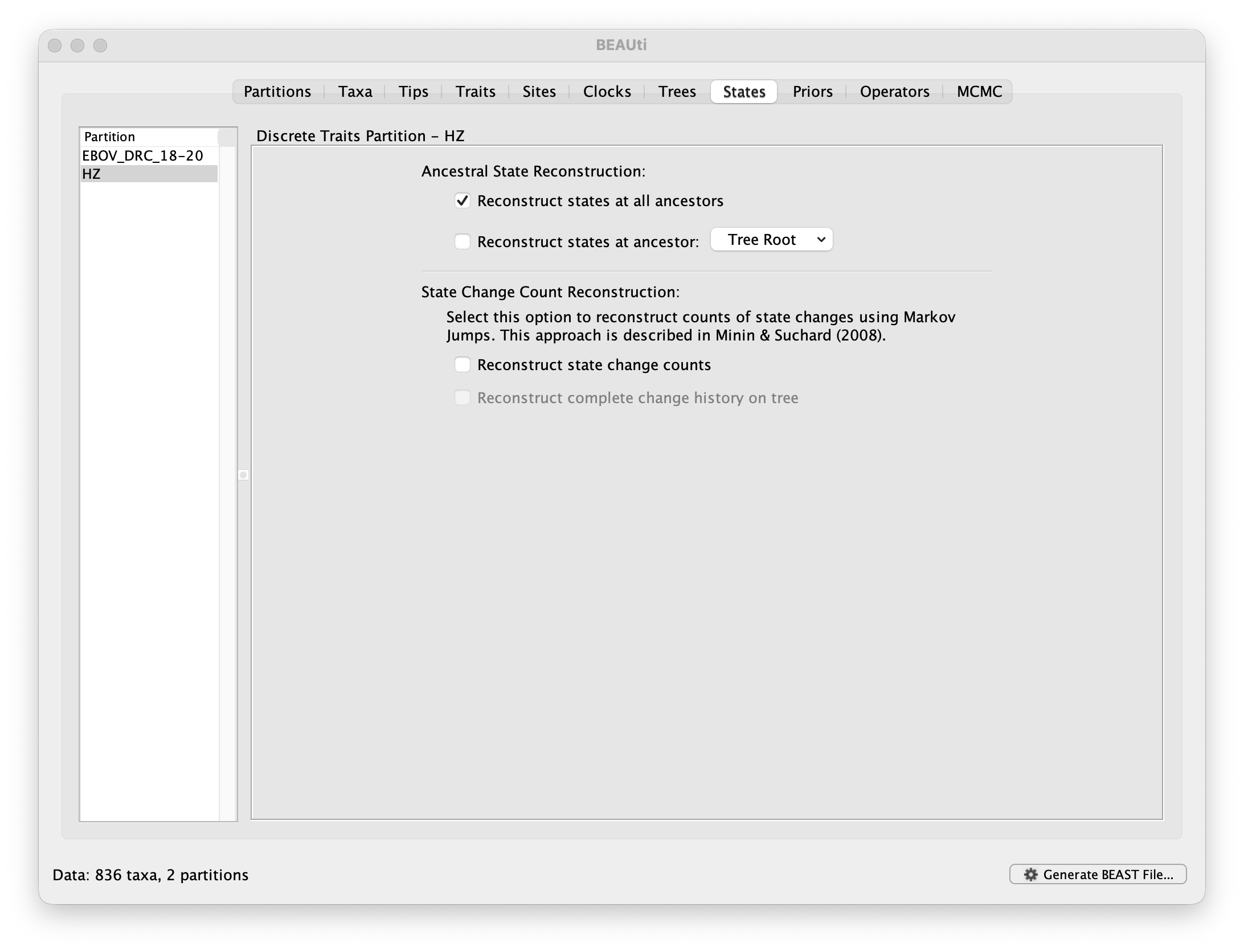
In the States panel, check that for HZ partition the option to Reconstruct states at all ancestors is selected (by default).
Setting up the priors
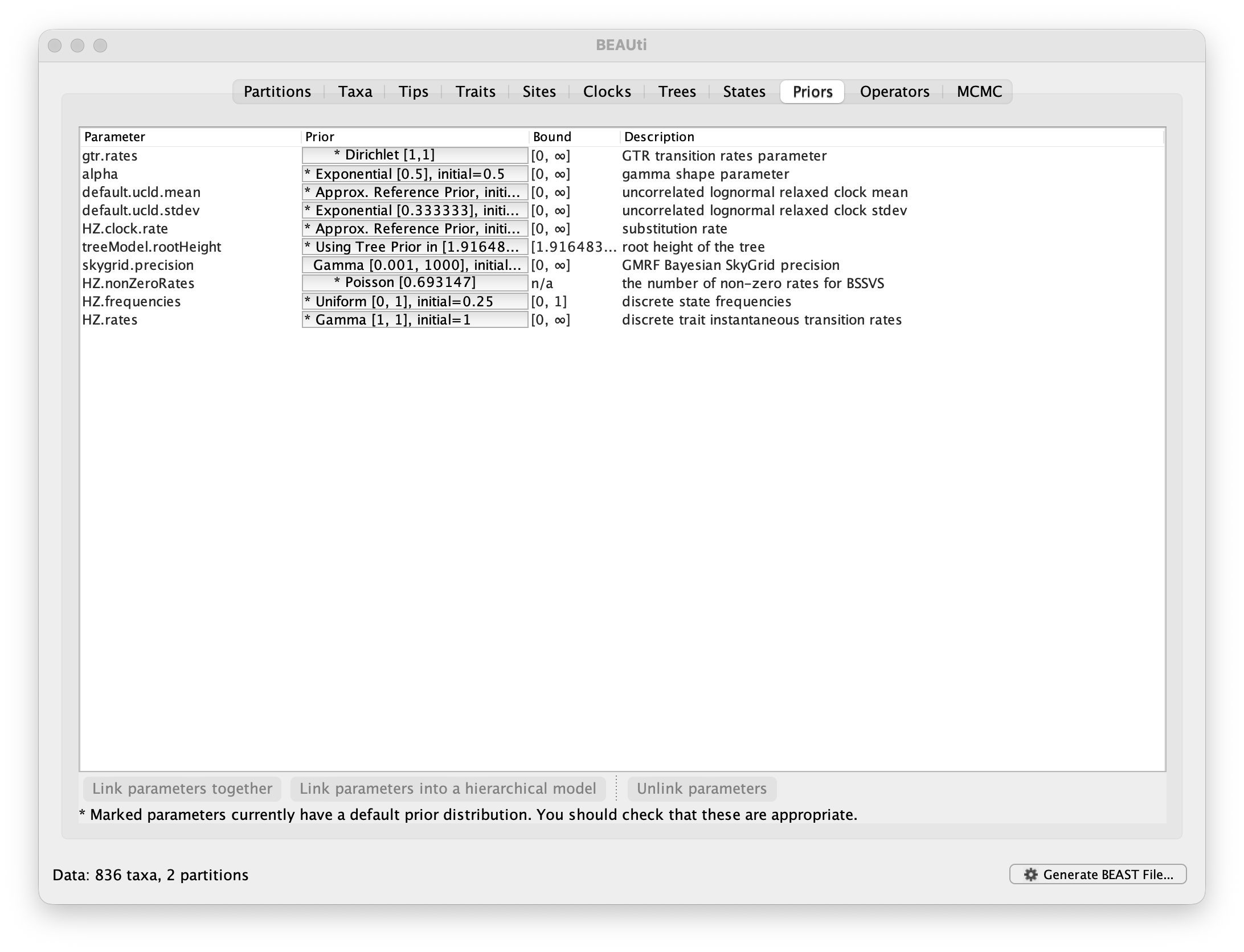
Now switch to the Priors tab. This panel has a table showing every parameter of the currently selected model and what the prior distribution is for each. A strong prior allows the user to ‘inform’ the analysis by selecting a particular distribution with a small variance. Alternatively we can select a weak (diffuse) prior to try to minimise the effect on the analysis. Note that a prior distribution must be specified for every parameter and whilst BEAUti provides default options these are not necessarily tailored to the problem and data being analyzed.
The default prior on the rate of evolution (default.ucld.mean) is an approximation of a conditional reference prior (Approx. Reference Prior) (Ferreira and Suchard, 2008). The same is applied to the discrete location state (HZ) rate. Note the Poisson prior specification for the BSSVS procedure (Gao et al., 2023).
Setting up the operators
Each parameter in the model has one or more “operators” (these are variously called moves, proposals or transition kernels by other MCMC software packages such as MrBayes and LAMARC). The operators specify how the parameters change as the MCMC runs. The Operators tab in BEAUti has a table that lists the parameters, their operators and the tuning settings for these operators:
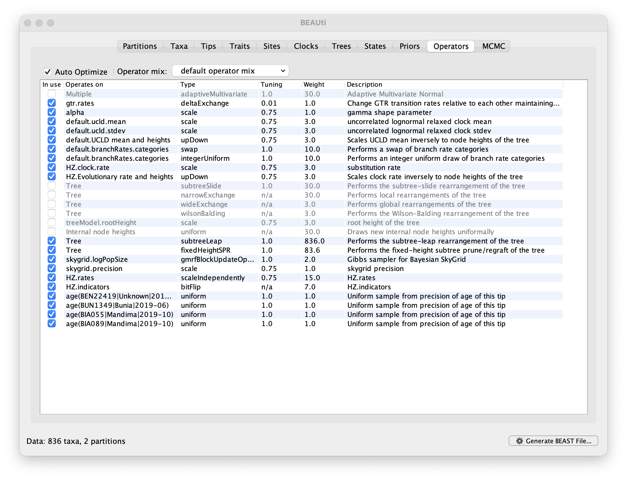
We can keep the default operator settings for the current analysis.
Setting the MCMC options
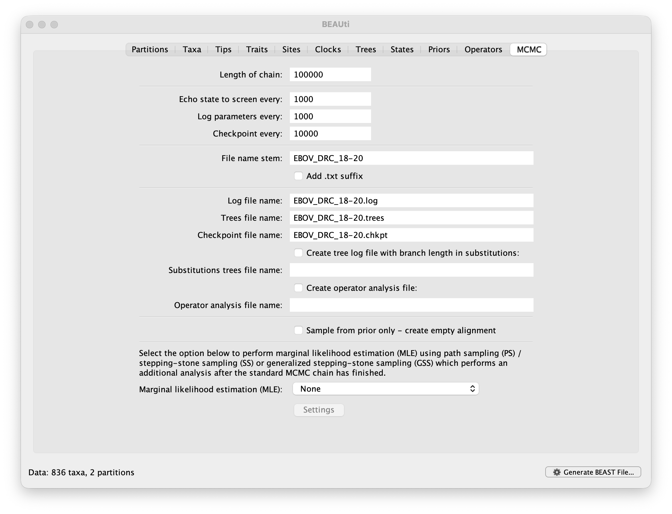
The MCMC tab in BEAUti provides settings to control the MCMC chain and the log files that get produced.
For this dataset let’s initially set the chain length to 100,000, both the sampling frequencies to 100 and checkpointing frequency to 10000. The File name stem: should already be set to EBOV_DRC_18-20 but you can adjust this (perhaps add more indications about the analysis).
We are now ready to create the BEAST XML file. Select Generate XML... from the File menu (or the button at the bottom of the window). BEAUti will ask you to review the prior settings one more time before saving the file (and will indicate if any are improper). Continue and choose a name for the file — it will offer the name you gave it in the MCMC panel and we usually end the filename with ‘.xml’ (although on Windows machines you may want to give the file the extension ‘.xml.txt’).
Running BEAST
Once the BEAST XML file has been created the analysis itself can be performed using BEAST.

Once BEAST has started a dialog box will appear in which you select the XML file:
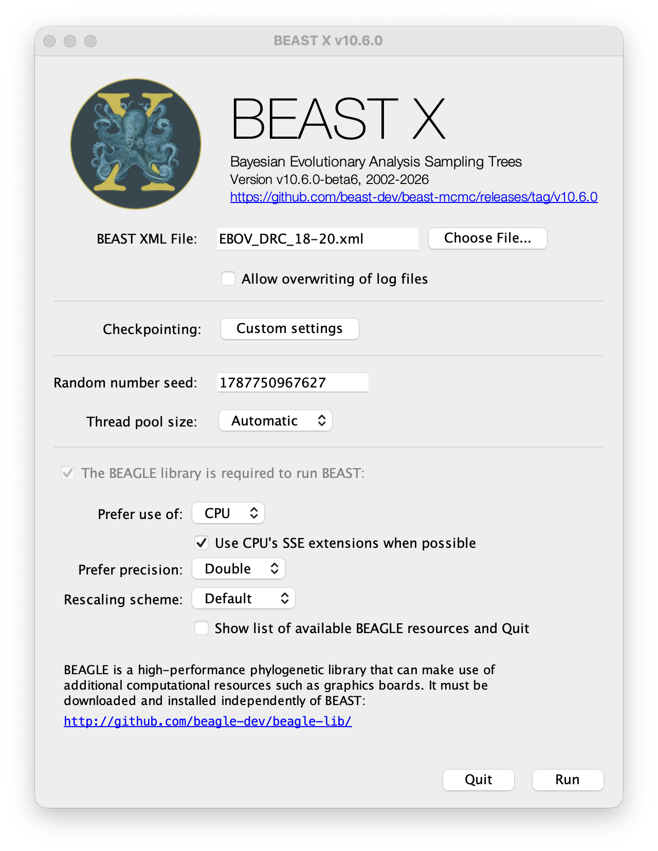
Press the Choose File... button and select the XML file you just created and press Run. The analysis will then be performed with detailed information about the progress of the run being written to the screen. When it has finished, the log file and the trees file will have been created in the same location as your XML file.
For more information about the other options in the BEAST dialog box see this page.
Analyzing the BEAST output using Tracer
To analyze the results of running BEAST we are going to use the program Tracer. The exact instructions for running Tracer differs depending on which computer you are using. Double click on the Tracer icon; once running, Tracer will look similar irrespective of which computer system it is running on.
Select the Import Trace File... option from the File menu. If you have the log file that you created in the previous section available, you could select this (EBOV_DRC_18-20.log). However, due to the data set size and discrete trait dimensionality, even the short chain will take some time to complete. So, if you do not wish to wait for this, you can go straight to selecting the log file from the longer run that has been made available (also EBOV_DRC_18-20.log).
Instead of importing trace files, you can also drag and drop your log file into the Tracer window. The file will load and you will be presented with a window similar to the one below. Remember that MCMC is a stochastic algorithm so the actual numbers will not be exactly the same.
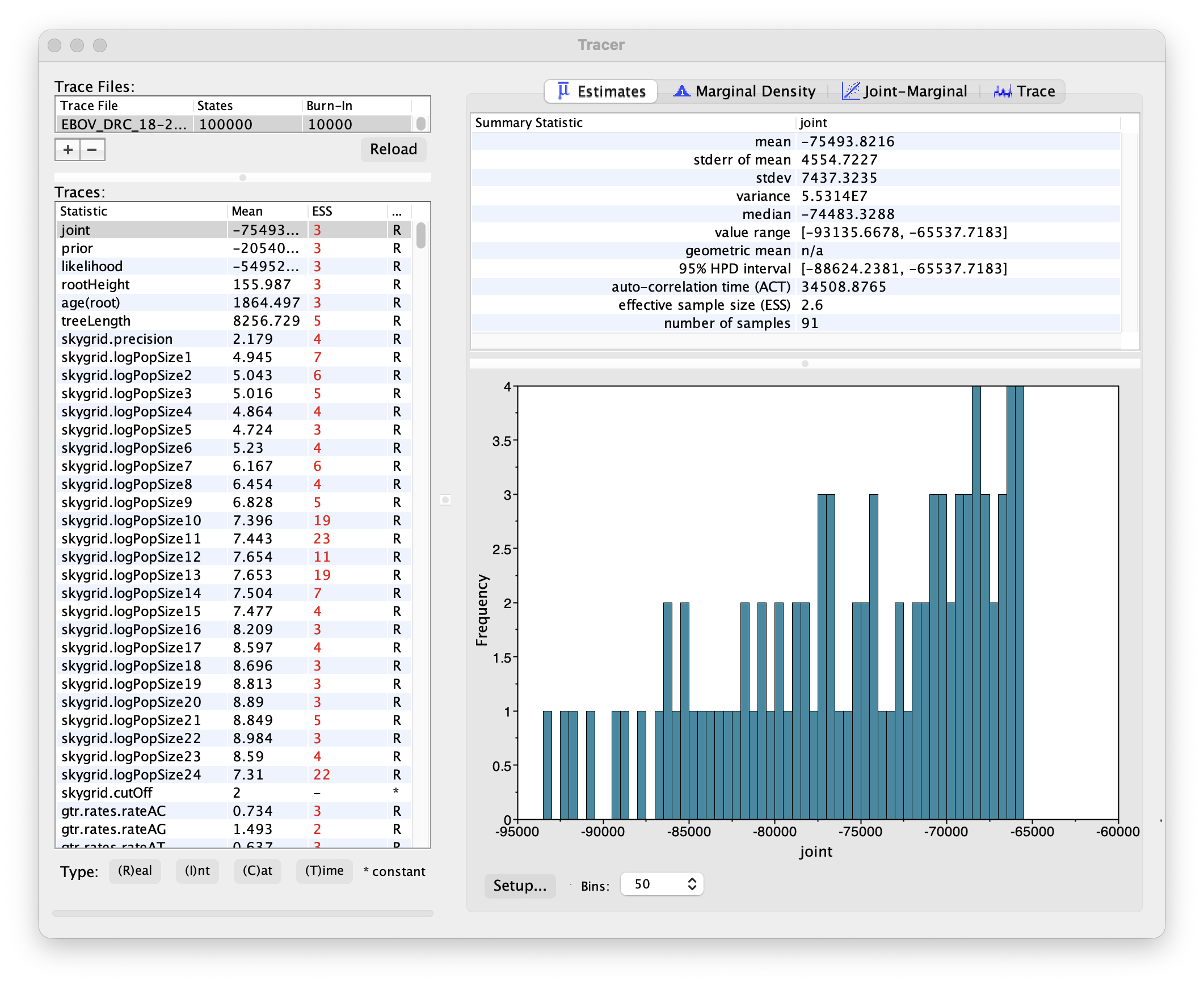
On the left hand side is the name of the log file loaded and the traces that it contains. There are traces for the posterior (joint, this is the log of the product of the tree likelihood and the prior probabilities), and the continuous parameters. Selecting a trace on the left brings up analyses for this trace on the right hand side depending on tab that is selected. When first opened, the ‘posterior’ trace is selected and various statistics of this trace are shown under the Estimates tab.
Note that the effective sample sizes (ESSs) for all the traces are very small. Select the Trace panel from the top of the window and inspecting the traces of the various parameters. You will see that the chain is still in the burn-in phase (the posterior values are still increasing over the entire chain), and this run does not allow us to summarize marginal posterior probability distributions for the parameters.
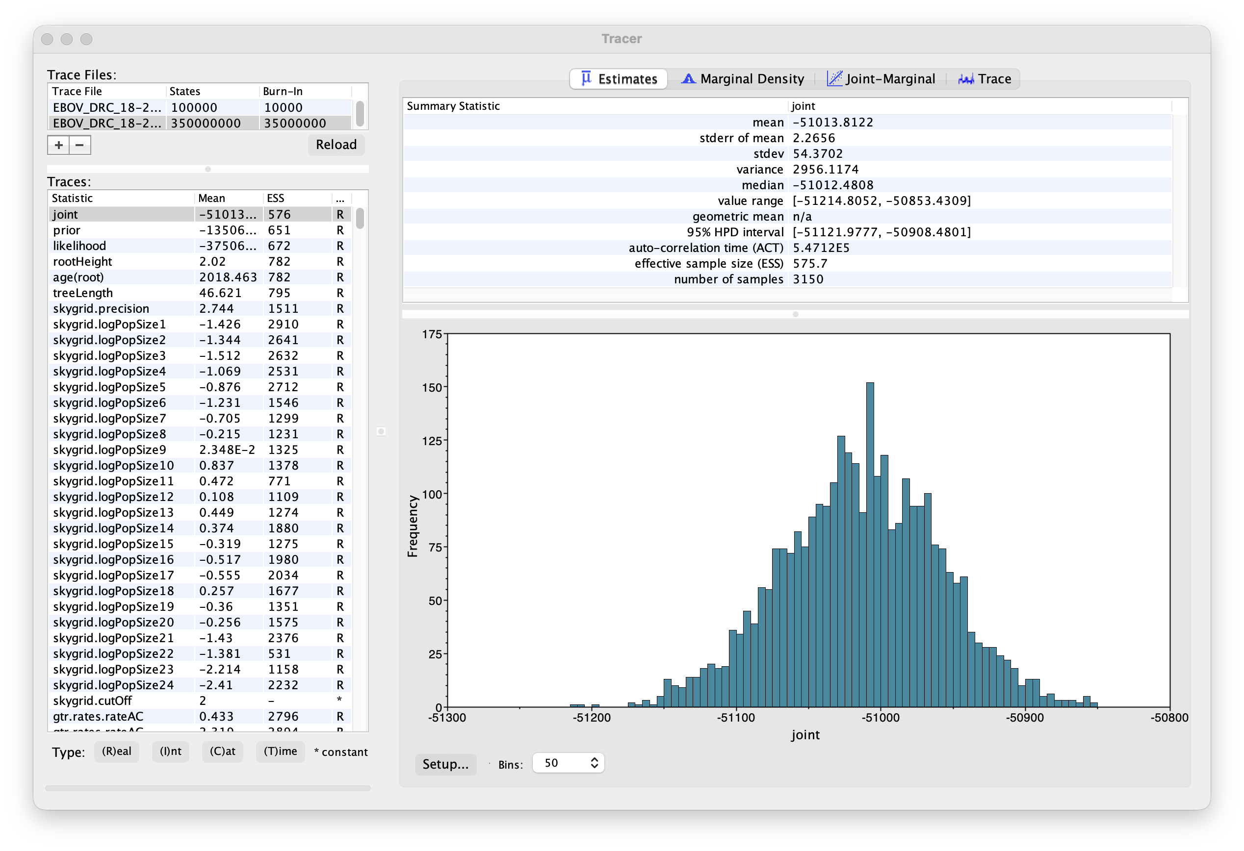
The simple response to this situation is that we need to run the chain for longer. We have provided the results of a very long run — 350 million steps, sampling every 100,000th step, resulting in 3,500 samples . In this case, the MCMC run has reached stationarity, and almost all parameter traces still show satisfactory ESSs. Only for the indicator variables, ESSs may still be low, but ESSs do not have the same interpretation for binary variables as compared to continuous variables.
You can load the long run log file (EBOV_DRC_18-20.log) into the same Tracer window for comparison to the short run. This gives this:
We can continue to summarize the annotated phylogeographic tree inferred with the BSSVS procedure and estimate the most significant rates of diffusion. If you are only interested in summarizing the Bayes Factor rates from the BSSVS analysis and not in summarizing the tree from your run, jump to the last section of this tutorial entitled Visualizing tree and calculating Bayes factor support for rates using SPREAD4.
Summarizing and visualizing the trees
At this point you can summarize the sampled trees using the TreeAnnotator utility. Note that the trees file provided in the zipped folder has been thinned to every 3rd sample (1,167 trees) to keep the download manageable, so TreeAnnotator will report fewer trees than the 3,500 samples in the log file.
You can use either FigTree or PearTree to visualize a summary tree like a HIPSTR tree obtained with TreeAnnotator.
Here, we will use PearTree to show a tree colored according to the annotated health zone location estimate for each node and tip.
Under BRANCHES, select HZ as Colour by and keep the default Tableau as Palette.

Select the same HZ attribute for Colour by under NODE SHAPES:

and under TIP SHAPES:

Finally, also show HZ under LEGEND:

This should result in a similar visualization as this one:

Visualizing the consensus tree using SpreadGL
SpreadGL, i.e. Spatial Phylogenetic Reconstruction of EvolutionAry Dynamics built on kepler.gl, is a software to visualize the output from Bayesian phylogeographic analysis and constitutes a user-friendly application to analyze and visualize reconstructions resulting from Bayesian inference of sequence and trait evolutionary processes. SpreadGL allows to visualise spatial reconstructions on custom maps and is run entirely online in browsers such as Firefox, Safari and Chrome.
To place the health zones on a map, SpreadGL needs a coordinate for each of them. The centroid of every health zone in the analysis is provided in healthzone_centroids.csv, a comma-separated file with one row per health zone and the columns health_zone, longitude and latitude.
EXERCISE 2: Identifying predictors for the spatial dispersal process
Background
This exercise builds on the previous analysis and aims at testing covariates associated with the spatiotemporal diffusion process. For this purpose, we adopt an extension of the discrete diffusion model that parameterizes the CTMC matrix as a generalized linear model (GLM), in which log CTMC rates are a log linear function of several potential predictors (most of the detail on the model can be found in Lemey et al., 2014). We explore a small set of relatively simple predictors: population size and geographic distance. Together, these can represent a so-called gravity model, which has been shown before as characteristic of EBOV spread (Dudas et al., Nature, 2017, 544, 309–315).
GLM-diffusion model specification
In case the BEAUti session from the previous exercise has not been closed yet, simply go back to the Sites panel. If it has been closed, repeat the first BEAUti steps up to specify the model settings up to those in the Sites panel. For the ‘HZ’ trait under Substitution Model, select Generalized Linear Model:
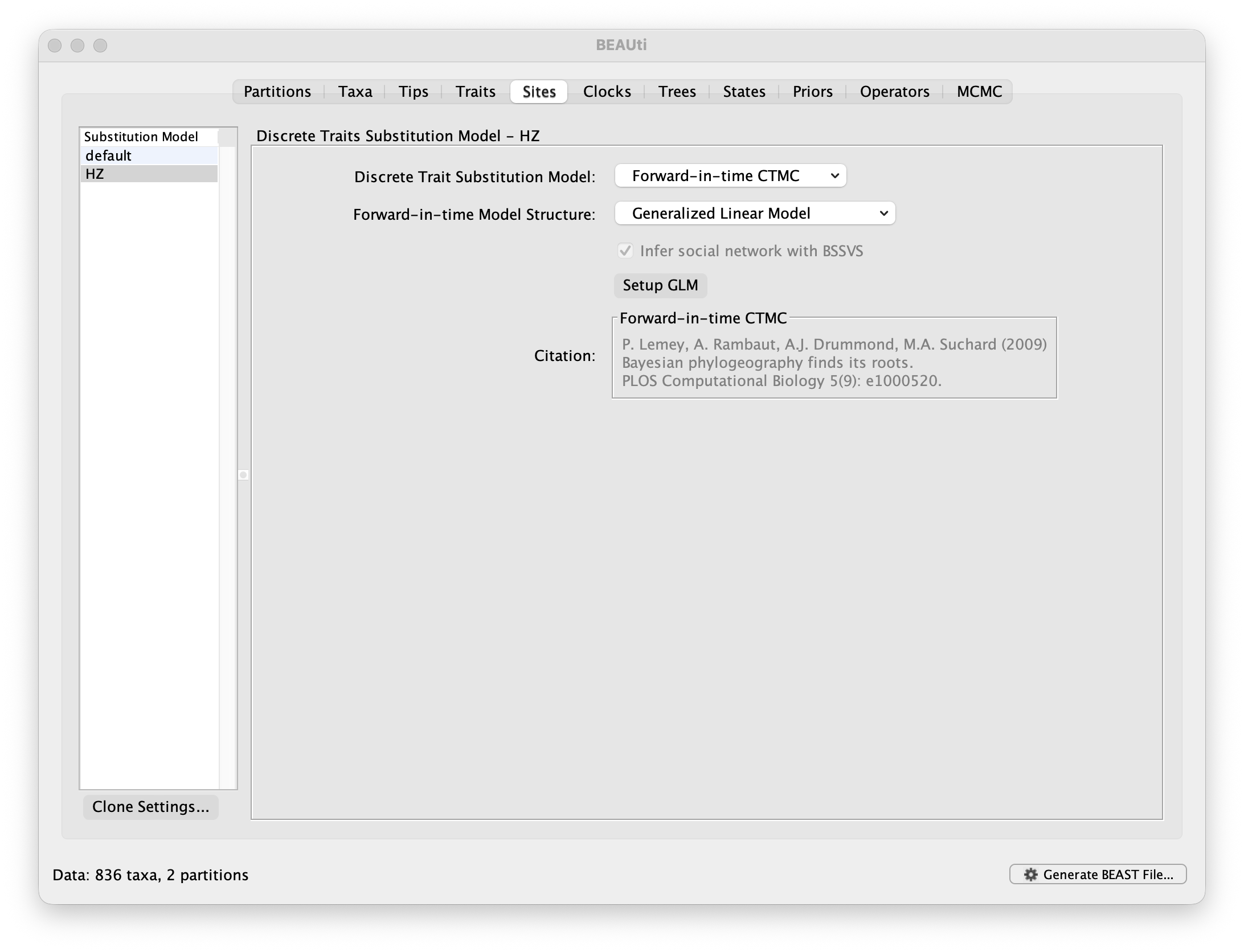
Click on Setup GLM and a new window will pop up:
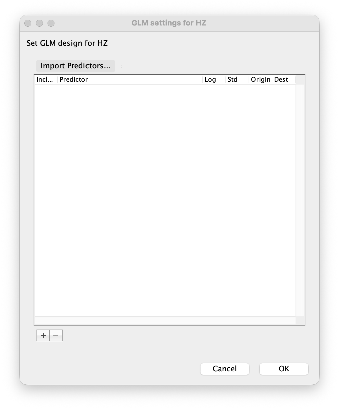
This window allows specifying a set of GLM predictors or covariates by importing them through Import Predictors....
Start by loading the population sizes through Import Predictors.... This is a csv file with the following content:
	HZ,pop_2019
	Alimbongo,235304
	Ariwara,211050
	Beni,408065
	Biena,126776
	Bunia,281153
	Butembo,337394
	Goma,268616
	Kalunguta,212947
	Katwa,438943
	Kayna,374825
	Komanda,193793
	Kyondo,229589
	Lolwa,48003
	Lubero,284071
	Mabalako,198636
	Mambasa,100565
	Mandima,144909
	Manguredjipa,77297
	Masereka,189583
	Musienene,266100
	Mutwanga,264633
	Mwenga,142408
	Nyankunde,102707
	Nyiragongo,462362
	Oicha,358713
	Rwampara,140581
	Vuhovi,129673
Note that by default, location-specific values like population sizes are used to construct both an Origin and Destination predictor. For the Origin version, the origin values are used to populate a pairwise matrix, while the destination values are used to populate a pairwise matrix of the Destination version. By default, these values are also log-transformed and standardised. This is because the GLM-diffusion model parameterizes the log of the CTMC rates as a log linear function of the predictor and we grant the same variance to the predictors a priori.
Next, load the geographic distances. This csv file contains pairwise great-circle distances between the centers of the health zones. As these already represent pairwise values, it is treated as a single covariate.
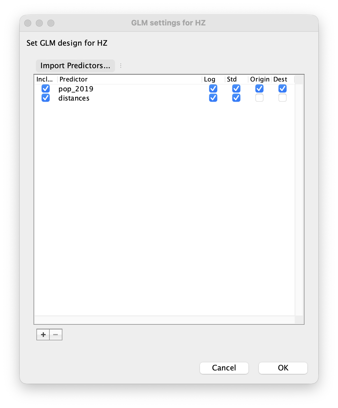
Proceed with the next steps as in the previous exercise. Note that in the Priors panel, a normal prior with mean 0 and a standard deviation of 2 is specified on the log GLM coefficients (‘HZ.coefficients’). We can again set up a short test run (e.g. 100,000 MCMC iterations), but proceed with diagnosing and summarising a long run. You can download the output of an MCMC analysis that has been run for 250 million iterations sampled every 50,000 generations:here.
Analyzing the GLM-diffusion model output
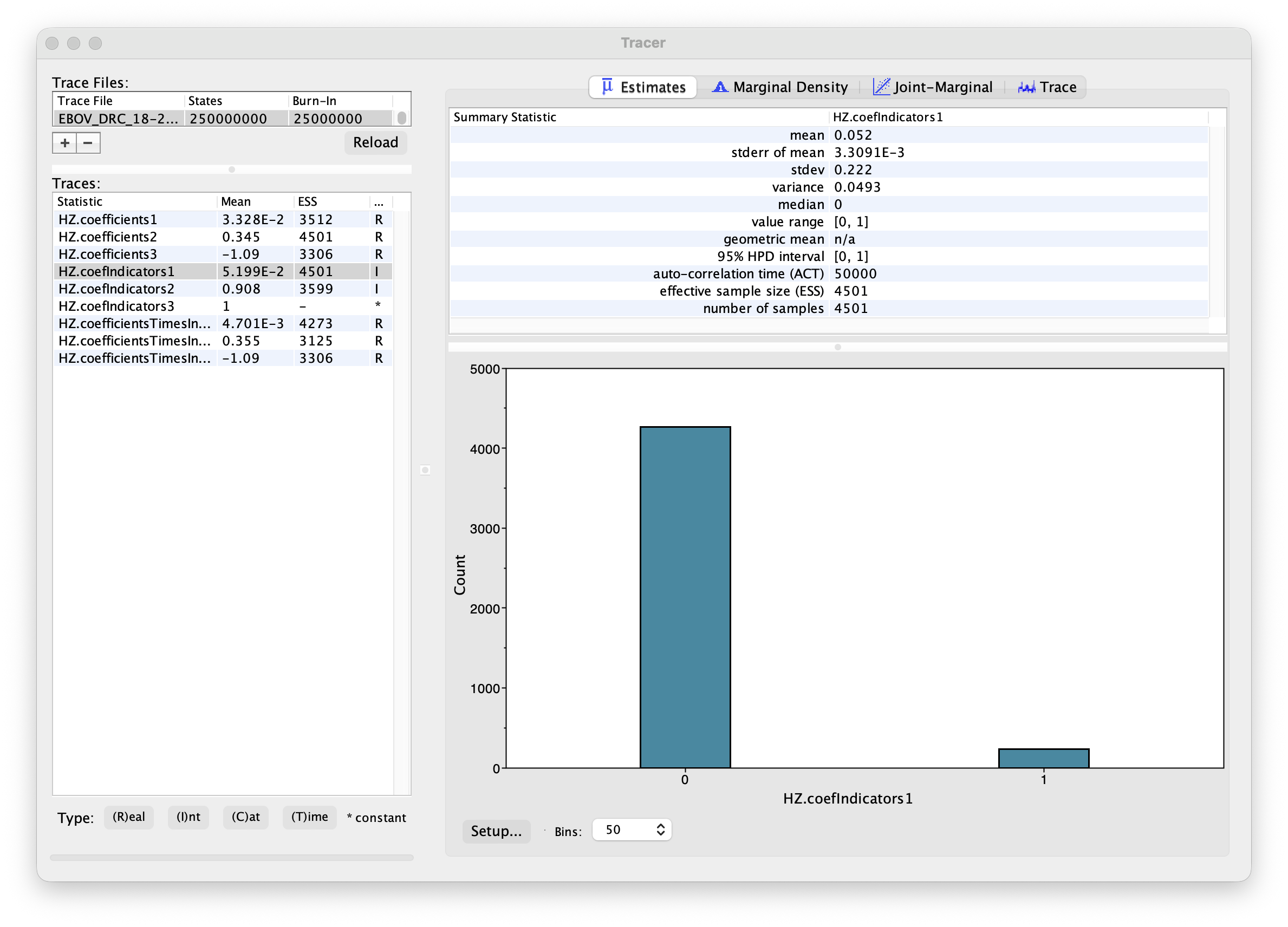
The parameters of interest in this analysis are the indicators associated with the predictors (‘HZ.coefIndicators1’ to ‘HZ.coefIndicators3’) and the coefficient parameters or effect sizes (‘HZ.coefficients1’ to ‘HZ.coefficients3’). Upon loading the log file (‘EBOV_DRC_18-20.HZ.glm.log’), the mean of an indicator provides an estimate for the inclusion probability of that indicator. In this case, the mean indicator for ‘HZ.coefIndicators1’, which represents the origin population size, is 0.052 implying that this predictor is only rarely included in the model. In contrast, the destination population size predictor (‘HZ.coefIndicators2’) has a posterior inclusion probability of 0.908 implying that this predictor is included in over 90% of the posterior samples. The distance predictor (‘HZ.coefIndicators3’) achieves maximum posterior inclusion probability and is therefore also included in the analysis.
In order to assess the evidence provided by the data for a predictor inclusion, we need to take into account the prior probability for inclusion. By default, BEAUti specifies Bernoulli prior probability distributions on these indicators with a small prior probability on each predictor’s inclusion, equivalent to a 50% prior probability on no predictors being included.
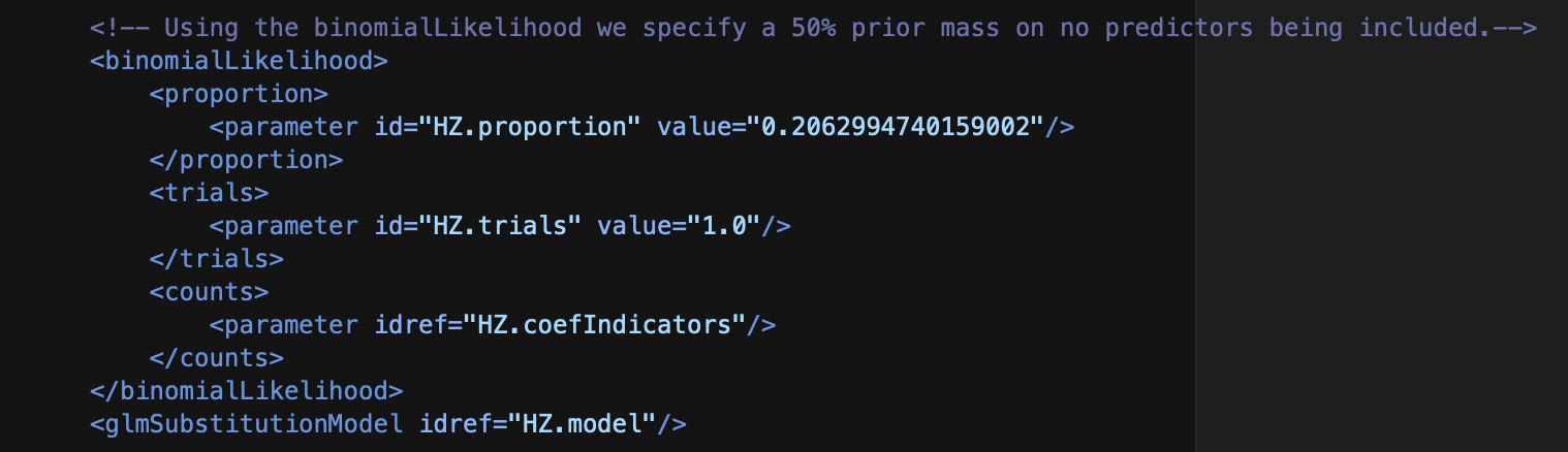
Based on both prior and posterior inclusion probabilities, we can calculate formal inclusion support in the form of Bayes Factors as these can be expressed as the ratio of the posterior odds over the prior odds for predictor inclusion. For an inclusion probability of 1, the Bayes factor is estimated as +infinity. In this case, it would be better to express the Bayes factor as being larger than X, where X would be the Bayes factor value if one sample had an indicator value of 1. For destinations population size, the posterior odds is 0.908/(1-0.908) = 9.870 while the prior odds is 0.206/(1-0.206) = 0.259; this results in a Bayes factor support value for the predictor inclusion of about 38. The origin population size predictor has a posterior inclusion probability smaller than its prior inclusion probability, so it will have Bayes factor < 1.
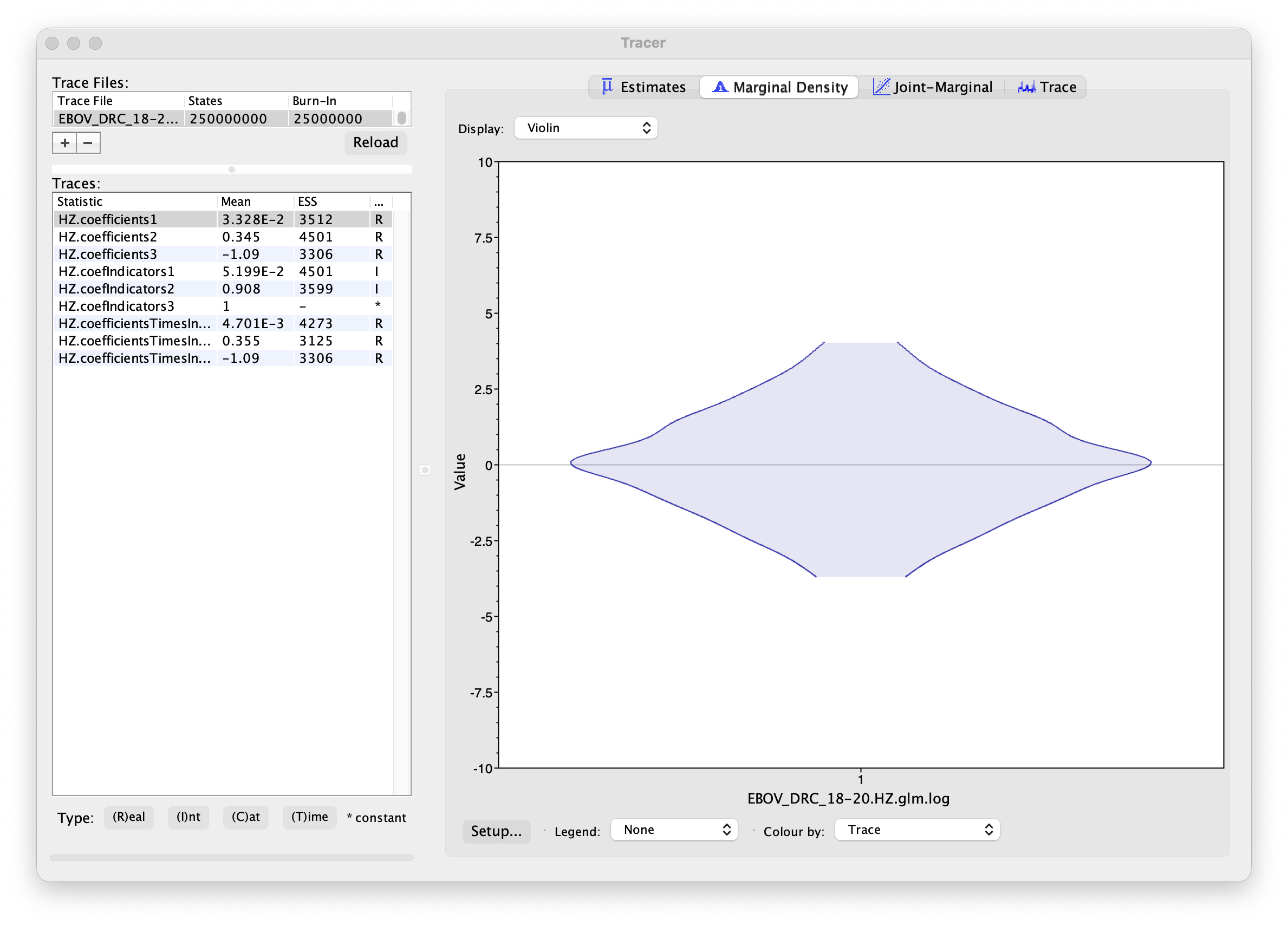
In order to assess the size of the contribution of predictors, we can use the estimates of the coefficients in log space. However, it is important to keep in mind that the estimates are critically dependent on the corresponding indicator value. If the indicator is 1, then the predictor is included in the model and the coefficient will be informed by the data (the predictor and the discrete states). If the indicator is 0, the predictor is not included and the coefficient value will be sampled from the prior. This is why posterior estimates of coefficients with very small inclusion probability will resemble the prior distribution (a normal distribution centered on 0 with a standard deviation of 2), as is the case for origin population size (‘HZ.coefficients1’). This is demonstrated by the violin plot for this coefficient in Tracer:
This may complicate the interpretation of coefficient estimates for predictors with intermediate inclusion probability. This is why applications have resorted to reporting the conditional effect size, that is the effect size when the predictor is included in the model (indicator = 1). In other words, this can be obtained by only summarising the coefficient estimates based on the samples for which the corresponding indicator values are 1. Alternatively, the predictor-specific product of the coefficient and indicator for all the samples can be summarised (these are logged as a statistic: HZ.coefficientsTimesIndicators1 to HZ.coefficientsTimesIndicators3). The violin plots for these statistics in Tracer look as follows:
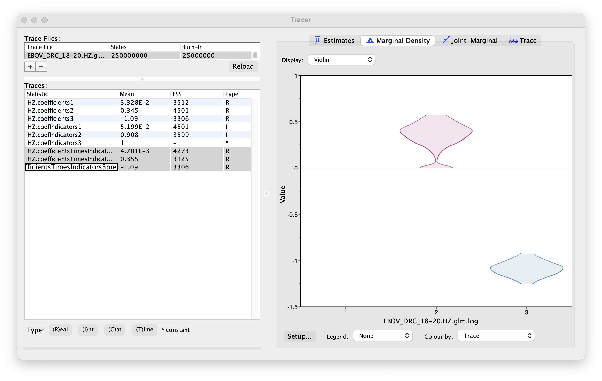
For geographic distance (‘HZ.coefficientsTimesIndicators3’), the posterior density for this statistic is the same as for the actual coefficient (‘HZ.coefficients3’) because the associated indicator is always 1 for this predictor. The negative coefficient provides evidence for a higher intensity of dispersal between nearby health zones. The posterior distribution for the statistic for destination population size (‘HZ.coefficientsTimesIndicators2’) shows most of its density on positive values but also a small density at 0, as expected for its inclusion probability. So, although this predictor does not yield maximum support as the geographic distances, it does suggest more intense dispersal towards more populated health zones.
EXERCISE 3: discrete ancestral reconstruction using the BASTA structured coalescent approximation (SCA)
In this exercise, we aim to perform a similar discrete ancestral reconstruction as in EXERCISE 1 but with a different model, i.e. a structured coalescent approximation known as BASTA (De Maio et al., 2015). Recent developments in computational efficiency for this model (Shao et al., 2026) now enable employing BASTA on moderately-sized data sets. Note however that, due to its design, a BASTA analysis using a backward-in-time model will run markedly slower compared to using the model in EXERCISE 1.
Running BEAUti
If your BEAUti window is still open from going through Exercise 1 above, you can go back to the Sites panel; if not, you can repeat the BEAUti steps from Exercise 1 until you reach the Sites panel. Select the trait HZ(for health zone) on the left-hand side and select the Backward-in-time CTMC model that is used in the BASTA SCA (see De Maio et al., 2015; Shao et al., 2026).
Specifying the trait information
In the Sites panel, Click on ‘HZ’ in the Substitution model window and choose the Backward-in-time CTMC model as Discrete Trait Substitution Model, Constant population size as the Backward-in-time Coalescent Model (currently the only option), and the Asymmetric substitution model as Backward-in-time Model Structure. Select the option to perform BSSVS (Infer social network with BSSVS), which enables the Bayesian Stochastic Search Variable Selection procedure, and also select Share coalescent model across demes which reduces the number of free parameters in the model to ensure identifiability (see e.g. De Maio et al., 2015; Shao et al., 2026).

Setting the ‘molecular clock’ model
We keep a Strict clock for the location partition, as it only contains a single column of data and hence more complicated clock models may lead to overfitting the data.
Setting the tree prior
Structured coalescent approximations make a direct link between the migration process and the population size dynamics at the demes, and hence there is no possibility to make a choice in this panel:

The ancestral states settings
In the States panel, check that for HZ partition the option to Reconstruct states at all ancestors is selected (by default). Note that there are fewer options than for the forward-in-time model in EXERCISE 1, but this will change in due time when Markov jumps for the BASTA model are developed.

Setting up the priors
The Priors panel has a table showing every parameter of the currently selected model and what the prior distribution is for each. A prior distribution must be specified for every parameter and whilst BEAUti provides default options these are not necessarily tailored to the problem and data being analyzed.
The default prior on the rate of evolution (default.ucld.mean) is an approximation of a conditional reference prior (Approx. Reference Prior) (Ferreira and Suchard, 2008). The same is applied to the discrete location state (HZ) rate. We here keep the prior specification of Lemey et al. (2009) for the BSSVS procedure.

Setting up the operators
Each parameter in the model has one or more “operators” (these are variously called moves, proposals or transition kernels by other MCMC software packages such as MrBayes and LAMARC). The operators specify how the parameters change as the MCMC runs. The Operators tab in BEAUti has a table that lists the parameters, their operators and the tuning settings for these operators:

We can keep the default operator settings for the current analysis.
Setting the MCMC options
In the MCMC tab, we keep the initial chain length to 100,000 (although for the BASTA model on this data set, ), both the sampling frequencies to 100 and checkpointing frequency to 10000. The File name stem: will still be set to EBOV_DRC_18-20 but you can easily adjust it to (for example): EBOV_DRC_18-20_BASTA.

We are now ready to create the BEAST XML file. Select Generate XML... from the File menu (or the button at the bottom of the window). BEAUti will ask you to review the prior settings one more time before saving the file (and will indicate if any are improper). Continue and choose a name for the file — it will offer the name you gave it in the MCMC panel and we usually end the filename with ‘.xml’ (although on Windows machines you may want to give the file the extension ‘.xml.txt’).
Running BEAST
Now that you have created another BEAST XML file, you can run the corresponding analysis in BEAST.
Once BEAST has started a dialog box will appear in which you select the XML file:

Press the Choose File... button and select the XML file you just created and press Run. The analysis will then be performed with detailed information about the progress of the run being written to the screen. When it has finished, the log file and the trees file will have been created in the same location as your XML file.
For more information about the other options in the BEAST dialog box see this page.
Analyzing the BEAST output using Tracer
While the analysis in the provided .log file has only run for 10 million iterations, it’s already interesting to take a look at what can be seen in Tracer.
Select the Import Trace File... option from the File menu. If you have the log file that you created in the previous section available, you could select this (EBOV_DRC_18-20_BASTA.log). However, due to the data set size and the choice of the BASTA structured coalescent model, even the short chain will take some time to complete. So, if you do not wish to wait for this, you can go straight to selecting the log file from the longer run that has been made available (also EBOV_DRC_18-20_BASTA_10m.log).
Instead of importing trace files, you can also drag and drop your log file into the Tracer window. The file will load and you will be presented with a window similar to the one below. Remember that MCMC is a stochastic algorithm so the actual numbers will not be exactly the same.
Tracer by default uses a burn-in of 10%, which here translates to 1 million iterations. This is clearly not enough, but we get an indication that an increased burn-in of 4 million iterations - based solely on the trace plot of the joint density - could be a reasonable first choice:

However, when we take a look at the traces for different parameters (e.g. the tree length) we note a clear downward trend, meaning that the analysis is likely still converging to the posterior:

Analyzing the BEAST output using TreeTracer
It’s interesting that the trace plot of the joint density in Tracer already seemed fairly stable after only 4 million iterations. Let’s have a look in TreeTracer (Hong et al., 2026) if the chain has already converged in phylogenetic tree space. There are two tutorials on TreeTracer readily available: TreeTracer tutorial 1 and TreeTracer tutorial 2. Launch TreeTracer, load the EBOV_DRC_18-20_BASTA_10m.trees file, and click the Compute RF distances and Compute MDS buttons:

Moving over to the Within-run Analysis panel confirms the burn-in of at least a few million iterations we observed in Tracer, and this in each pairwise 2D projection (MDS1 x MDS2, MDS1 x MDS3, MDS2 x MDS3) of the MDS; (very) light blue dots represent tree samples from the start of the analysis, whereas dark blue samples represent the latest trees sampled from the Markov chain:

We can obtain a more objective confirmation of a lack of tree convergence and mixing with the sample and its current burn-in setting by checking the Diagnostics panel. First click the Compute RF Trace button, followed by the Compute Tree-ESS button. The different trace plots that will appear confirm that we need to modify the burn-in when inspecting the stored tree samples. Further, the tree ESS - similar to the ESS values in Tracer for continuous parameters, but for phylogenetic trees - is colored red (indicating a Fréchet correlation ESS far below the threshold of 500; Magee et al., 2024) and hence indicates that we need to reassess our current burn-in setting and (very likely) the current chain length:

It’s hence a good idea to go back to the Compute Distances panel and set a burn-in of 400 tree samples, leaving 601 tree samples to be analysed. You don’t have to restart the TreeTracer application to do this, but you can if you find this to be easier. Click the Compute RF distances and Compute MDS buttons to recompute all metrics and visualisations with this updated burn-in setting:

When we now inspect the Within-run Analysis panel, we no longer observe the initial convergence in the different 2D projections of the MDS. However, we can still clearly see a pattern in the first two projections (MDS1 x MDS2 and MDS1 x MDS3) that may indicate the burn-in setting was not set sufficiently high:

This is more clearly visible in the 3D visualisation of the MDS, which you can find in the Between-run Analysis panel:

In conclusion, this BASTA phylogeographic analysis needs to be run for (much) longer to be able to perform a more in-depth assessment of convergence and mixing in phylogenetic tree space. Based on what Tracer and TreeTracer show for the initial 10 million iterations, it would seem that at least 50 or 100 million iterations will be required to perform a more informative inspection of convergence and mixing for the continuous model parameters (in Tracer) and the sampled phylogenetic trees (in TreeTracer).
Once such an analysis for possibly hundreds of millions of iterations has been completed, the same steps as in EXERCISE 1 (Summarizing and visualizing the trees and Visualizing the consensus tree using SpreadGL) can then be followed to compare the consensus tree obtained under the BASTA model to the one obtained in EXERCISE 1 under a forward-in-time (FIT) CTMC model. Note that the Compare Consensus panel in TreeTracer offers the possibility to compare consensus trees through a tanglegram, but see TreeTracer tutorial 1 for more information on how to do this. Finally, we refer to Baele et al. (2025) for a comparison of consensus tree methods, all of which are available in TreeAnnotator X.
References
- Kinganda-Lusamaki, E., Black, A., Mukadi, D.B. et al. 2021. Integration of genomic sequencing into the response to the Ebola virus outbreak in Nord Kivu, Democratic Republic of the Congo. Nat Med 27, 710–716. doi: 10.1038/s41591-021-01302-z
- Ferreira, M. A. R. and M. A. Suchard. 2008. Bayesian analysis of elapsed times in continuous-time Markov chains. Can J Statistics, 36: 355–368. doi: 10.1002/cjs.5550360302
- Lemey, P., A. Rambaut, A. J. Drummond, and M. A. Suchard. 2009. Bayesian phylogeography finds its roots. PLoS computational biology 5:e1000520.
- Lemey, P., A. Rambaut, T. Bedford, N. Faria, F. Bielejec, G. Baele, C. A. Russell, D. J. Smith, O. G. Pybus, D. Brockmann, and M. A. Suchard. 2014. Unifying Viral Genetics and Human Transportation Data to Predict the Global Transmission Dynamics of Human Influenza H3N2. PLoS pathogens 10:e1003932.
- Bloomquist, E. W., P. Lemey, and M. A. Suchard. 2010. Three roads diverged? Routes to phylogeographic inference. Trends Ecol Evol 25:626-632.## Help and documentation.
- Nahata KD, Bielejec F, Monetta J, Dellicour S, Rambaut A, Suchard MA, Baele G, Lemey P. 2022. SPREAD 4: online visualisation of pathogen phylogeographic reconstructions. Virus Evol., 26;8(2):veac088. doi: 10.1093/ve/veac088. eCollection 2022.
- De Maio N, Wu C.-H., O’Reilly K. M., Wilson D. 2015. New Routes to Phylogeography: A Bayesian Structured Coalescent Approximation. PLOS Genet. 11(8): e1005421.
- Shao Y., Suchard M. A., Rambaut A., Ji X, Lemey P, Vasylyeva T. I., Baele G. 2026. Parallel algorithms for phylogenetic inference under a structured coalescent approximation. Proc. Natl. Acad. Sci. USA 123 (18) e2602412123.
- Gao J., May M. R., Rannala B., Moore B. R. 2023. Model misspecification misleads inference of the spatial dynamics of disease outbreaks. Proc. Natl. Acad. Sci. USA 120 (11) e2213913120.
- Hong S. L., Brusselmans M., Klaps J., Carvalho L. M., Magee A. F., Suchard M. A., Rambaut A., Baele G. (2026) Tree convergence and mixing in Bayesian phylogenetics Using TreeTracer. In preparation.
- Magee A., Karcher M., Matsen IV F. A., Minin V. (2024) How trustworthy is your tree? Bayesian phylogenetic effective sample size through the lens of Monte Carlo error. Bayesian Analysis, 19(2), 565-593.
- Baele G., Carvalho L. M., Brusselmans M., Dudas G., Ji X, McCrone J. T., Lemey P., Suchard M. A., Rambaut A. (2025) HIPSTR: highest independent posterior subtree reconstruction in TreeAnnotator X. Bioinformatics 41(10): btaf488.
Help and documentation
The BEAST website: http://beast.community
Tutorials: http://beast.community/tutorials
Frequently asked questions: http://beast.community/faq