With sequence data
Loading the sequence data
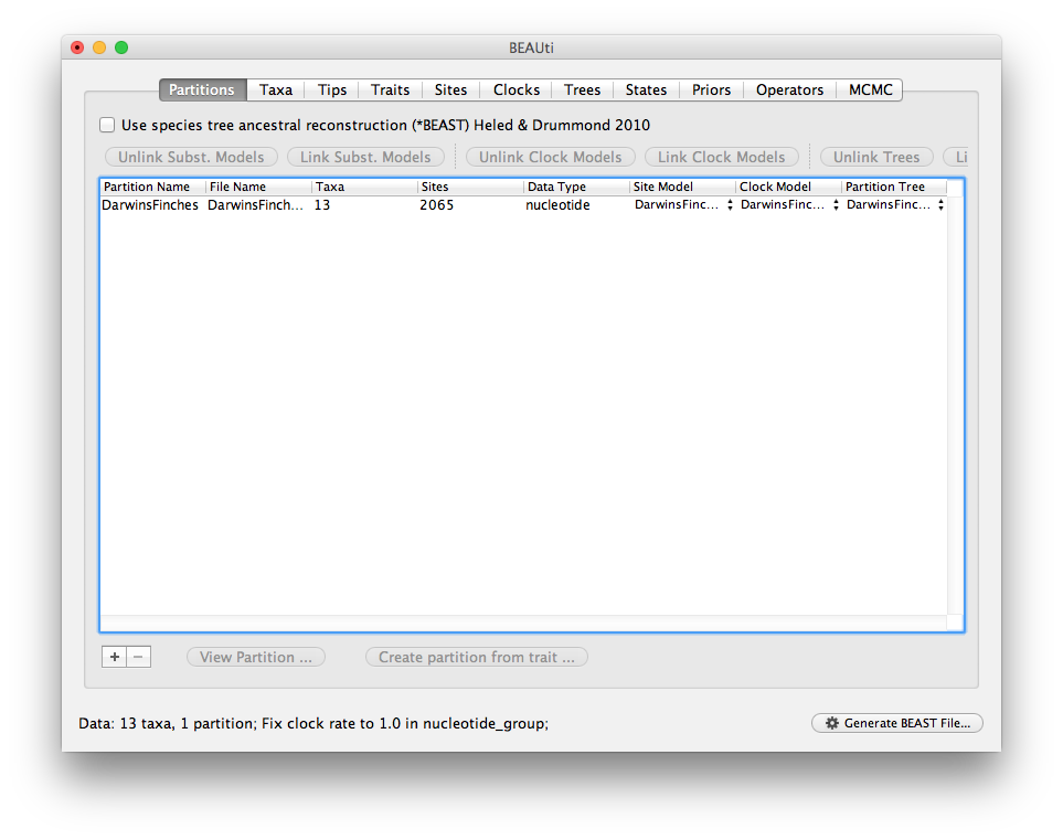
To load a NEXUS format alignment, simply select the Import Data... option from the File menu.
For this tutorial select the file in examples/continuousTraits/DarwinsFinches.nex in the BEAST package.
Once loaded the data panel will look like this:
Loading the trait data
Next import the trait data from the file examples/continuousTraits/DarwinsFinchesTraits.txt. This is a tab-delimited text file with the first column having taxon names (to match those in the sequence data) and each subsequent column having trait values. The first row contains the names of the traits (the first column of the first row is ignored and can be empty).
The data is as shown here:
| wingL | tarsusL | culmenL | beakD | gonysW | |
|---|---|---|---|---|---|
| Geospiza magnirostris | 4.4042 | 3.03895 | 2.724667 | 2.823767 | 2.675983 |
| Geospiza conirostris | 4.349867 | 2.9842 | 2.6544 | 2.5138 | 2.360167 |
| Geospiza difficilis | 4.224067 | 2.898917 | 2.277183 | 2.0111 | 1.929983 |
| Geospiza scandens | 4.261222 | 2.929033 | 2.621789 | 2.1447 | 2.036944 |
| Geospiza fortis | 4.244008 | 2.894717 | 2.407025 | 2.362658 | 2.221867 |
| Geospiza fuliginosa | 4.132957 | 2.806514 | 2.094971 | 1.941157 | 1.845379 |
| Cactospiza pallida | 4.265425 | 3.08945 | 2.43025 | 2.01635 | 1.949125 |
| Certhidea olivacea | 3.975393 | 2.936536 | 2.051843 | 1.191264 | 1.401186 |
| Camarhynchus parvulus | 4.1316 | 2.97306 | 1.97442 | 1.87354 | 1.81334 |
| Camarhynchus pauper | 4.2325 | 3.0359 | 2.187 | 2.0734 | 1.9621 |
| Pinaroloxias inornata | 4.1886 | 2.9802 | 2.3111 | 1.5475 | 1.6301 |
| Platyspiza crassirostris | 4.419686 | 3.270543 | 2.331471 | 2.347471 | 2.282443 |
| Camarhynchus psittacula | 4.23502 | 3.04912 | 2.25964 | 2.23004 | 2.07394 |
DarwinsFinchesTraits.txt
The actual file looks like this with the species name in the first column and the names of the traits in the first row. Each item is separated by a tab character:
	wingL	tarsusL	culmenL	beakD	gonysW
Geospiza magnirostris	4.4042	3.03895	2.724667	2.823767	2.675983
Geospiza conirostris	4.349867	2.9842	2.6544	2.5138	2.360167
Geospiza difficilis	4.224067	2.898917	2.277183	2.0111	1.929983
Geospiza scandens	4.261222	2.929033	2.621789	2.1447	2.036944
Geospiza fortis	4.244008	2.894717	2.407025	2.362658	2.221867
Geospiza fuliginosa	4.132957	2.806514	2.094971	1.941157	1.845379
Cactospiza pallida	4.265425	3.08945	2.43025	2.01635	1.949125
Certhidea olivacea	3.975393	2.936536	2.051843	1.191264	1.401186
Camarhynchus parvulus	4.1316	2.97306	1.97442	1.87354	1.81334
Camarhynchus pauper	4.2325	3.0359	2.187	2.0734	1.9621
Pinaroloxias inornata	4.1886	2.9802	2.3111	1.5475	1.6301
Platyspiza crassirostris	4.419686	3.270543	2.331471	2.347471	2.282443
Camarhynchus psittacula	4.23502	3.04912	2.25964	2.23004	2.07394
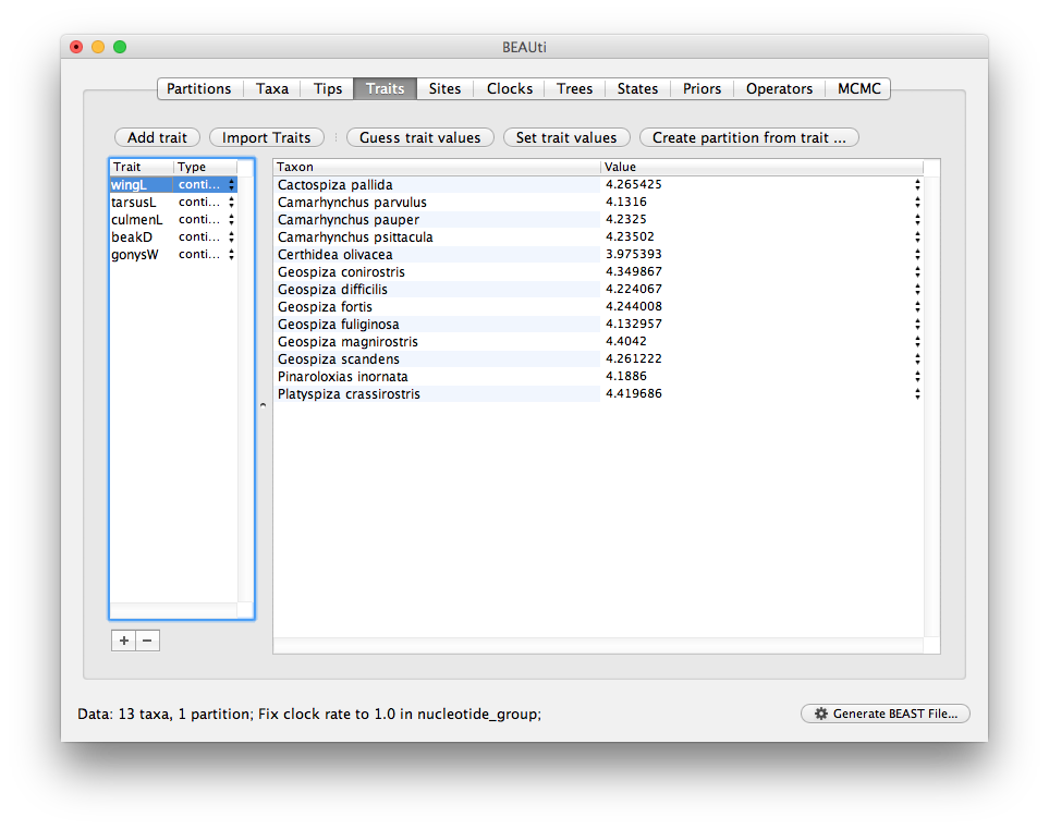
Select the Import Traits... option from the File menu.
Once loaded the trait panel will look like this:
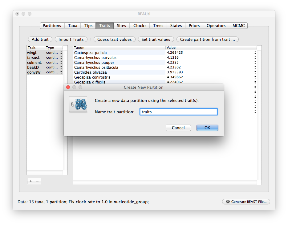
Next we need to combine the individual traits into a multivariate data partition.
Select all five traits in the table on the left and press the Create partition from trait... button.
You will be asked for a name for this new partition.
Give it the name ‘traits’ (or whatever is appropriate):
Setting up the models
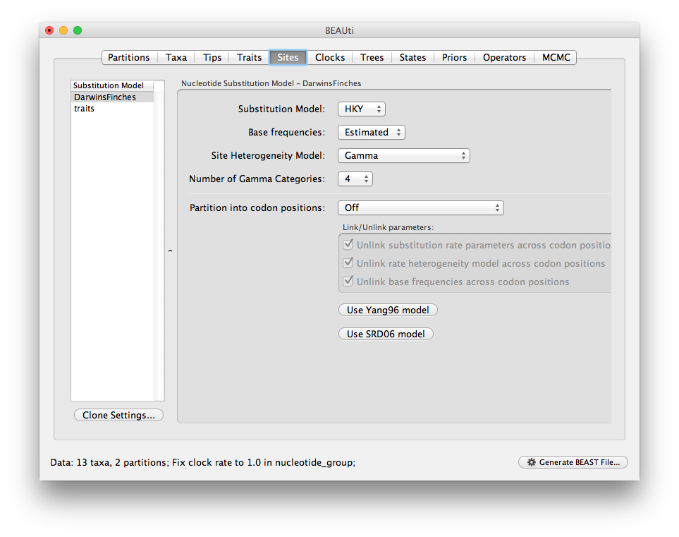
Switch to the Sites panel to select the evolutionary models for each data partition. You should see two data partitions, ‘DarwinsFinches’, the nucleotide data we loaded first, and ‘traits’, the multivariate trait partition we just created from the five traits (you should also see both partitions in the data table on the Data panel). Select your preferred nucleotide substitution model for the sequence data:
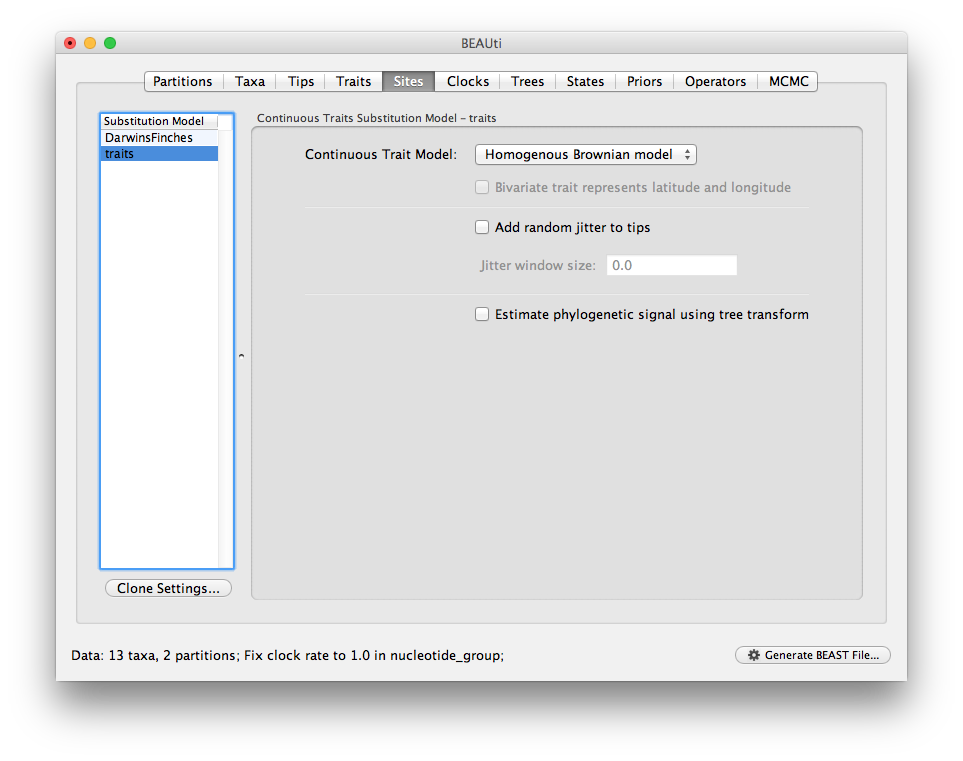
Now select the ‘traits’ partition and choose the continuous trait evolution model (in this case a Homogenous Brownian-motion model):
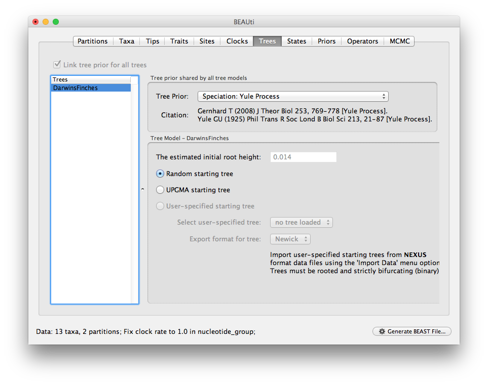
Now select other aspects of the model such as the tree prior model (such as the Yule model):
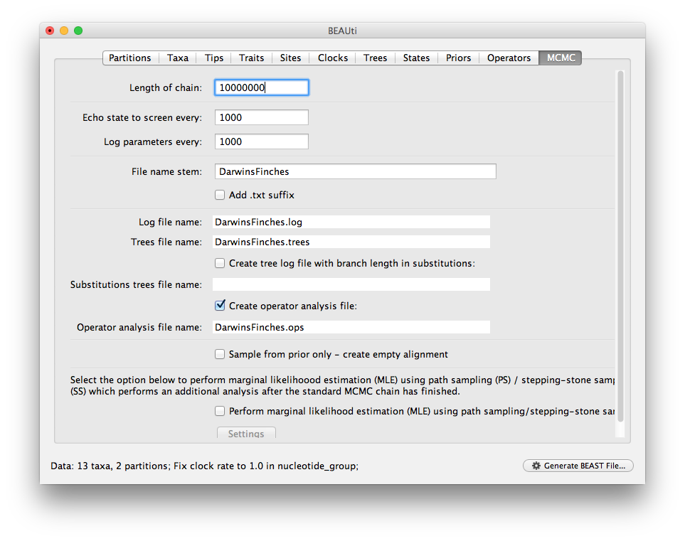
Choose a name stem for the output files and an appropriate chain length:
Analysing the data
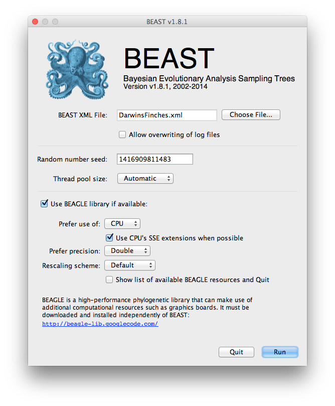
Then generate the XML file and load it into BEAST to run:
To analyse the results, the usual combination of Tracer and TreeAnnotator/PearTree can be used. Firstly load the log file into Tracer:
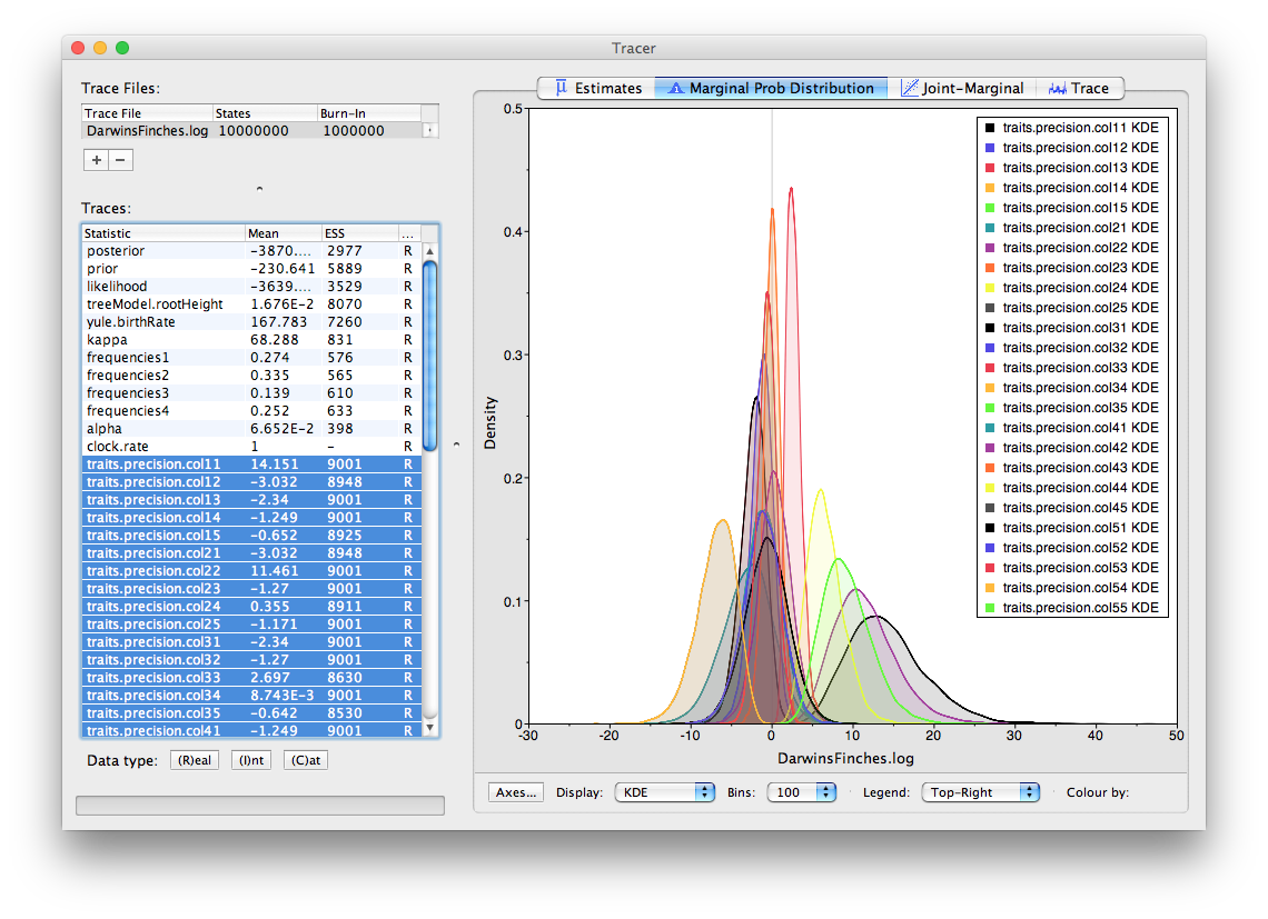
In the above, the traces labeled colXY are the precisions or co-precisions of the traits X and Y (in order they appeared in BEAUti). So, for the finch data, col11 is the precision of the first trait, ‘wingL’. Selecting all the precisions (i.e., col11, col22 etc.) we can see how much variation there is in the traits (precision being the reciprocal of the variance, the bigger the number the smaller the variance). Looking through all the co-precisions it is clear there is a strong negative value for trait 4 and 5 (beakD and gonysW). This is corresponds to a strong positive correlation (the variance/covariance matrix is the inverse of the precision matrix).
You can also construct a summary MCC tree using the TreeAnnotator tool and then visualise individual dimensions of the traits using PearTree (i.e., by colouring the branches). We currently don’t have any multivariate visualisation tools for these analyses but we hope to provide some in the future.