Introduction
The first step will be to convert a fasta file into a BEAST XML input file. This is done using the program BEAUti (this stands for Bayesian Evolutionary Analysis Utility). This is a user-friendly program for setting the evolutionary model and options for the MCMC analysis. The second step is to actually run BEAST using the input file that contains the data, model and settings. The final step is to explore the output of BEAST in order to diagnose problems and to summarize the results.
To undertake this tutorial, you will need to download three software packages in a format that is compatible with your computer system (all three are available for Mac OS X, Windows and Linux/UNIX operating systems):
EXERCISE 1: The transmission dynamics of SARS-CoV-2 alpha and omicron BA.1 in the U.K.
Running BEAUti
To load a fasta alignment, simply select the Import Data... option from the File menu.
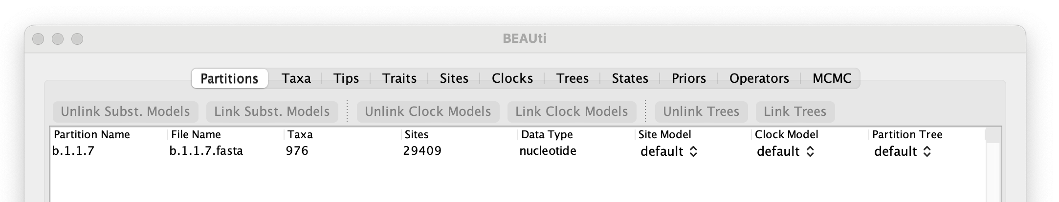
To start with the analysis of the alpha data set, select the file called b.1.1.7.fasta. This file contains an alignment of 976 genomes, 29,409 nucleotides in length. Once loaded, the new data will be listed under Partitions as shown in the figure:
Setting the tip dates
To undertake a phylodynamic analysis we need to specify the dates that the individual viruses were collected. In this case, the sequences were sampled between September and December 2020. To set these dates switch to the Tips panel using the tabs at the top of the window.
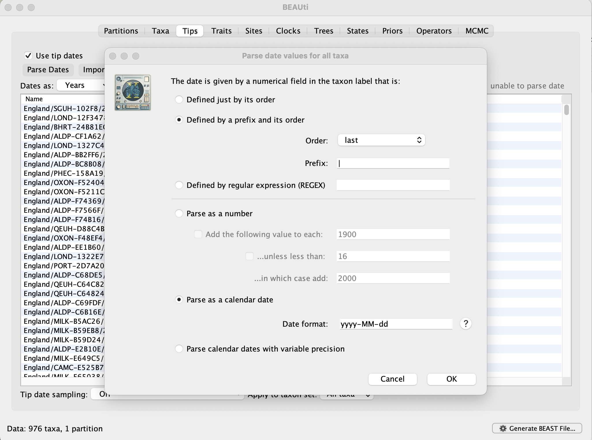
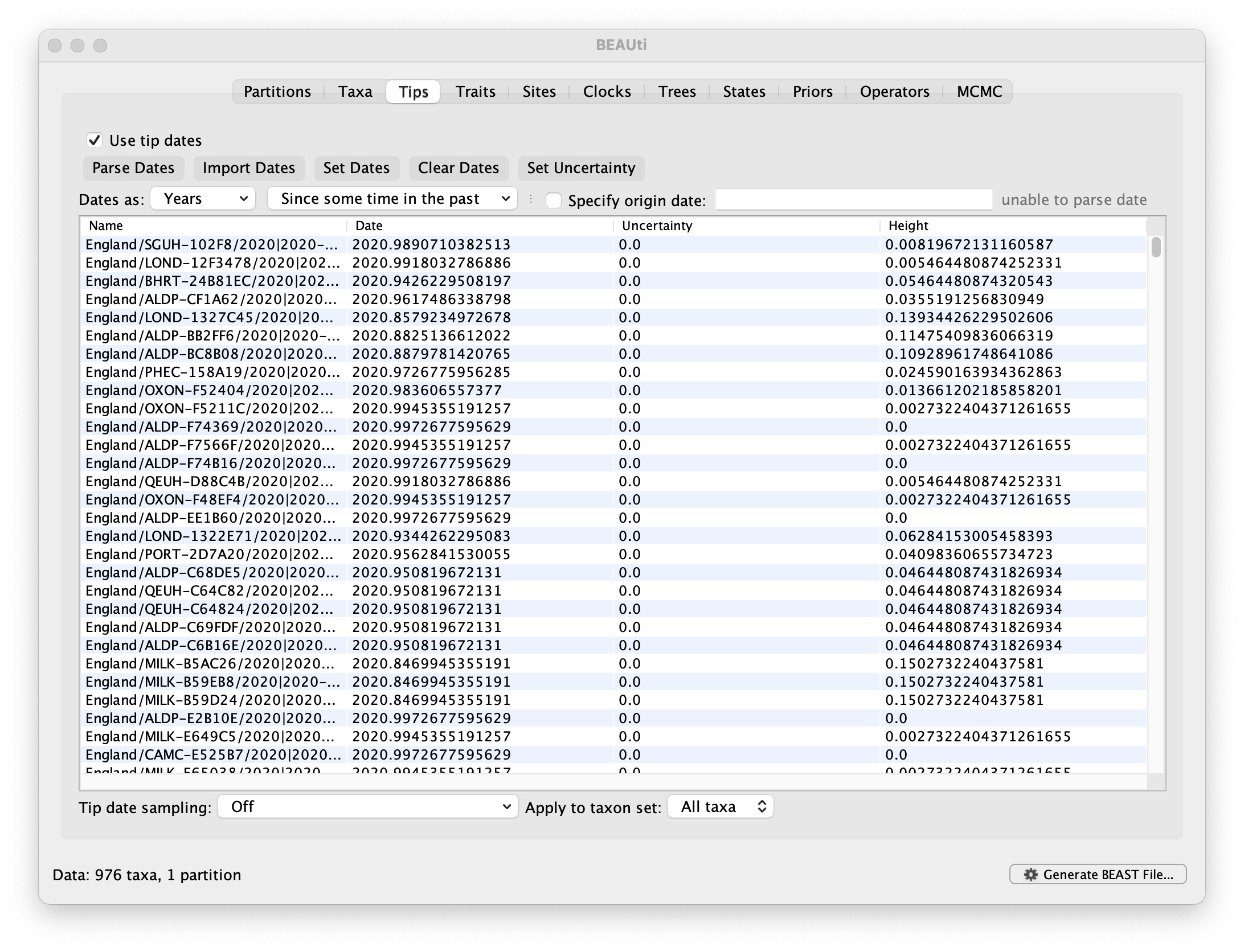
Select the box labelled Use tip dates. The actual sampling time is encoded in the name of each taxon (at the end, using the year-mm-dd format) and we can use the Parse Dates button at the top of the panel to extract these. For the alpha sequences, select the Defined by a prefix and its order option. Select last from the Order drop-down menu and enter the pipe symbol | as Prefix. Select the Parse as a calendar date (and keep the default Date format) and press OK. The dates will appear in the appropriate column of the main window. You can then check these and edit them manually in case this would be required.
Setting the substitution model
The next thing to do is to click on the Sites tab at the top of the main window to specify the evolutionary model settings for BEAST:
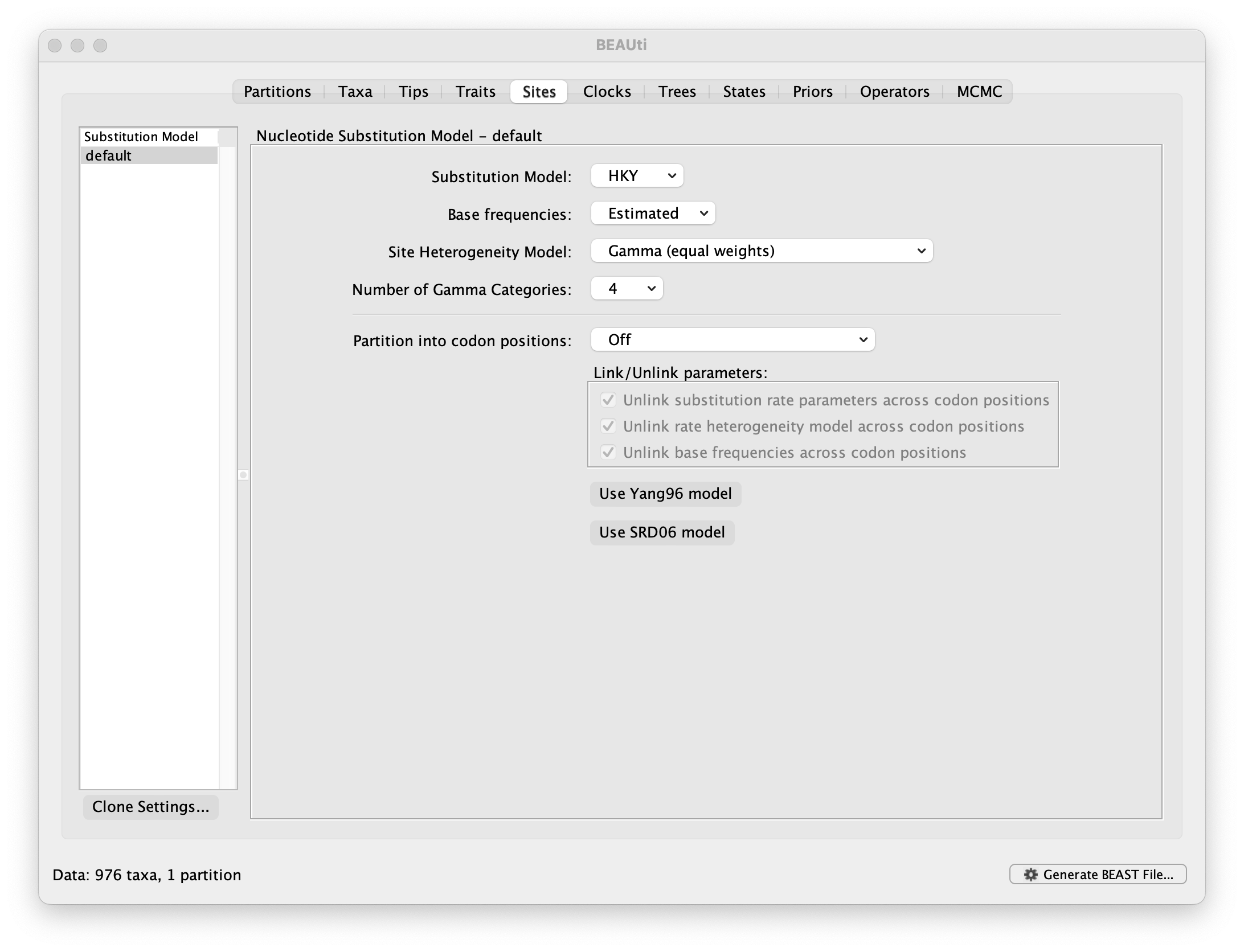
For this tutorial, keep the default HKY model, the default Estimated base frequencies and select Gamma (equal rates) as Site Heterogeneity Model (with 4 discrete categories) before proceeding to the Clocks tab.
Setting the molecular clock model
The Clocks panel options allows us to choose between a strict and a relaxed (uncorrelated lognormal or uncorrelated exponential) clock. Because of the low diversity data we analyze here and its limited sampling time range, a relaxed clock would probably be over-parameterization. Hence, we keep a strict clock setting.
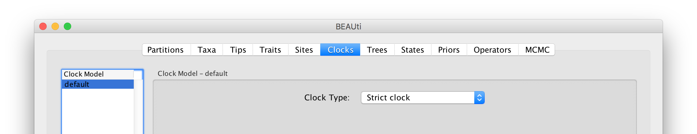
Now move on to the Trees panel.
Setting the tree prior
This panel contains settings about the tree. Firstly the starting tree is specified to be ‘randomly generated’. The other main setting here is to specify the Tree prior which describes how the population size is expected to change over time for coalescent models. The default tree prior is set to a constant size coalescent prior. The range of different tree priors (coalescent and other models) are described on this page.
To estimate the epidemic growth rate, we will change this demographic model to an exponential growth coalescent prior, which is intuitively appealing for viral outbreaks. Switch the option for Tree Prior to Coalescent: Exponential Growth:
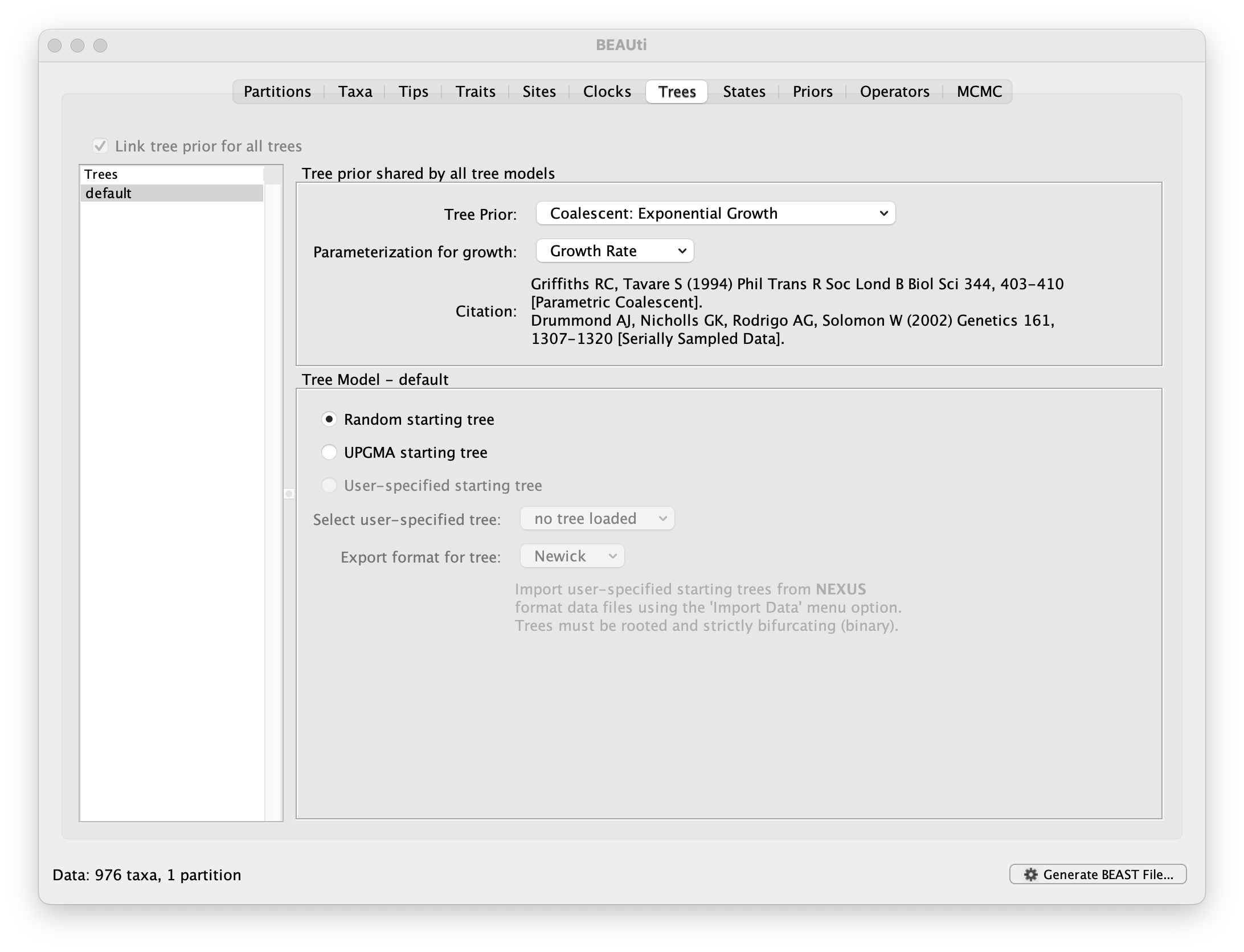
Note that the default parameterisation of the exponential growth coalescent model uses Growth Rate, but we can also opt for a parameterisation in terms of a Doubling time, which has an intuitive interpretation. We can also explore this parameterisation as an alternative later in this exercise (cfr. below). In either case, we can log the alternative statistic by checking the box when setting up this parameterization.
If the serial interval is known, we can therefore also calculate the R0 from the growth rate. Following Volz et al. (2021), we can use \(\mu = 6.44\) days and \(\sigma = 4.25\) days.
Setting up the priors
Now switch to the Priors tab. This panel has a table showing every parameter of the currently selected model and what the prior distribution is for each. A strong prior allows the user to ‘inform’ the analysis by selecting a particular distribution with a small variance. Alternatively we can select a weak (diffuse) prior to try to minimise the effect on the analysis. Note that a prior distribution must be specified for every parameter and whilst BEAUti provides default options these are not necessarily tailored to the problem and data being analyzed.
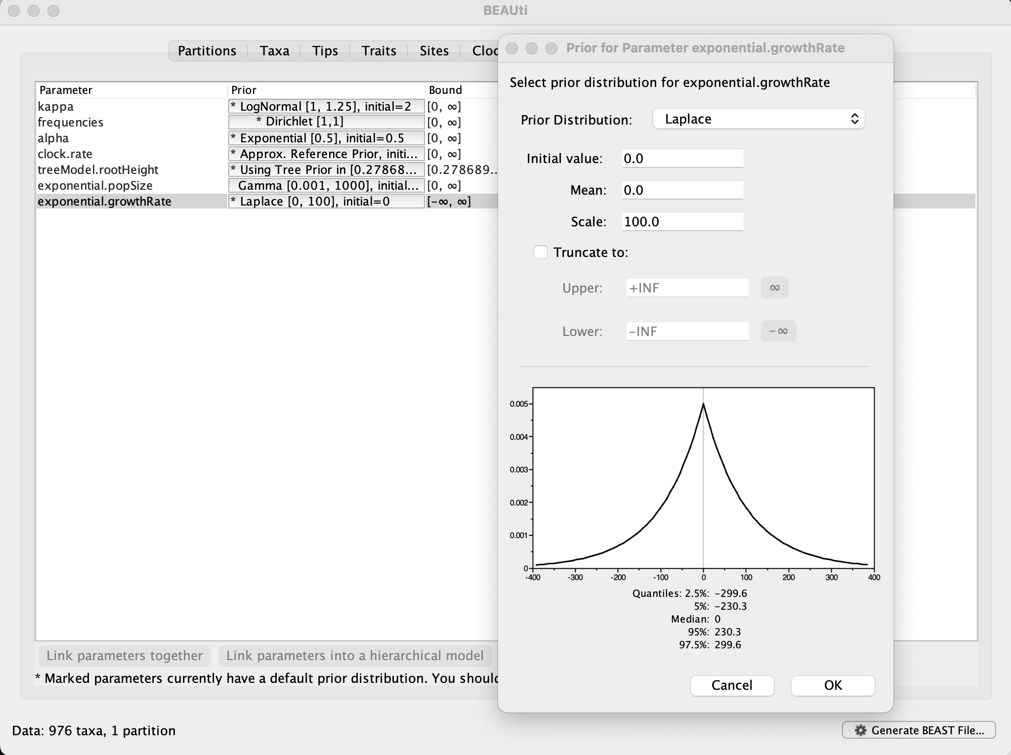
On this epidemic scale, the growth rate parameter take could take on relatively large values. Therefore, we will use the default scale of 100. However, depending on the analysis, a stronger prior and thus smaller variance could be preferred. A useful exercise could be to examine the sensitity of the growth rate estimates to different scale values for this prior distribution (e.g. scale = 1, 10, 100).
All the priors here can be left at their default options.
Setting up the operators
Each parameter in the model has one or more “operators” (these are variously called moves, proposals or transition kernels by other MCMC software packages such as MrBayes and LAMARC). The operators specify how the parameters change as the MCMC runs. The Operators tab in BEAUti has a table that lists the parameters, their operators and the tuning settings for these operators:
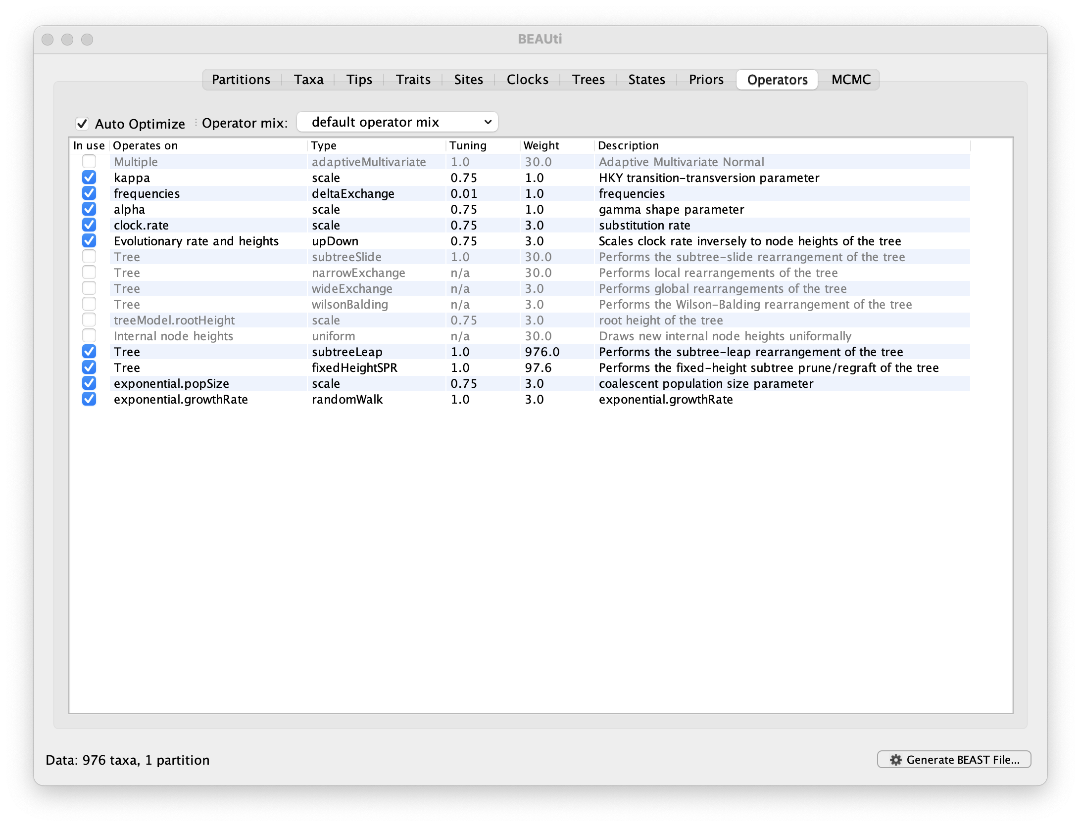
Notice that the coalescent growth rate parameter (exponential.growthrate) has a randomWalk operator. This is appropriate for a parameter that can take both positive and negative values (parameters that are strictly positive can use a scale operator). No changes are required in this table.
Setting the MCMC options
The MCMC tab in BEAUti provides settings to control the MCMC chain and the log files that get produced.
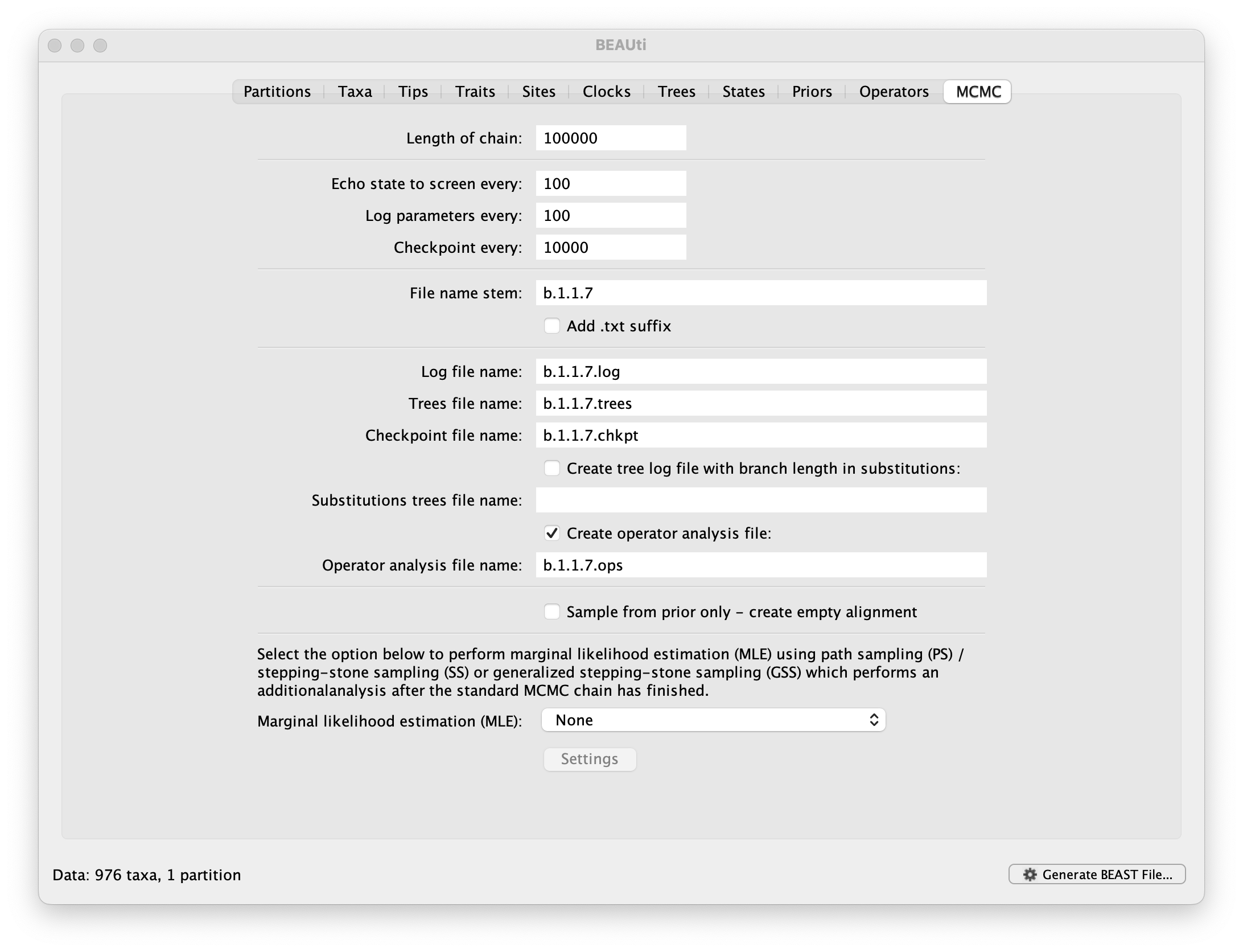
For this dataset let’s initially set the chain length to 100,000, both the sampling frequencies to 100 and the checkpointing frequency to .10000 The File name stem: should already be set to b.1.1.7 but you can adjust this (perhaps add more indications about the analysis).
We are now ready to create the BEAST XML file. Select Generate XML... from the File menu (or the button at the bottom of the window). BEAUti will ask you to review the prior settings one more time before saving the file (and will indicate if any are improper). Continue and choose a name for the file — it will offer the name you gave it in the MCMC panel and we usually end the filename with ‘.xml’ (although on Windows machines you may want to give the file the extension ‘.xml.txt’).
Running BEAST
Once the BEAST XML file has been created the analysis itself can be performed using BEAST.
Once BEAST has started a dialog box will appear in which you select the XML file:
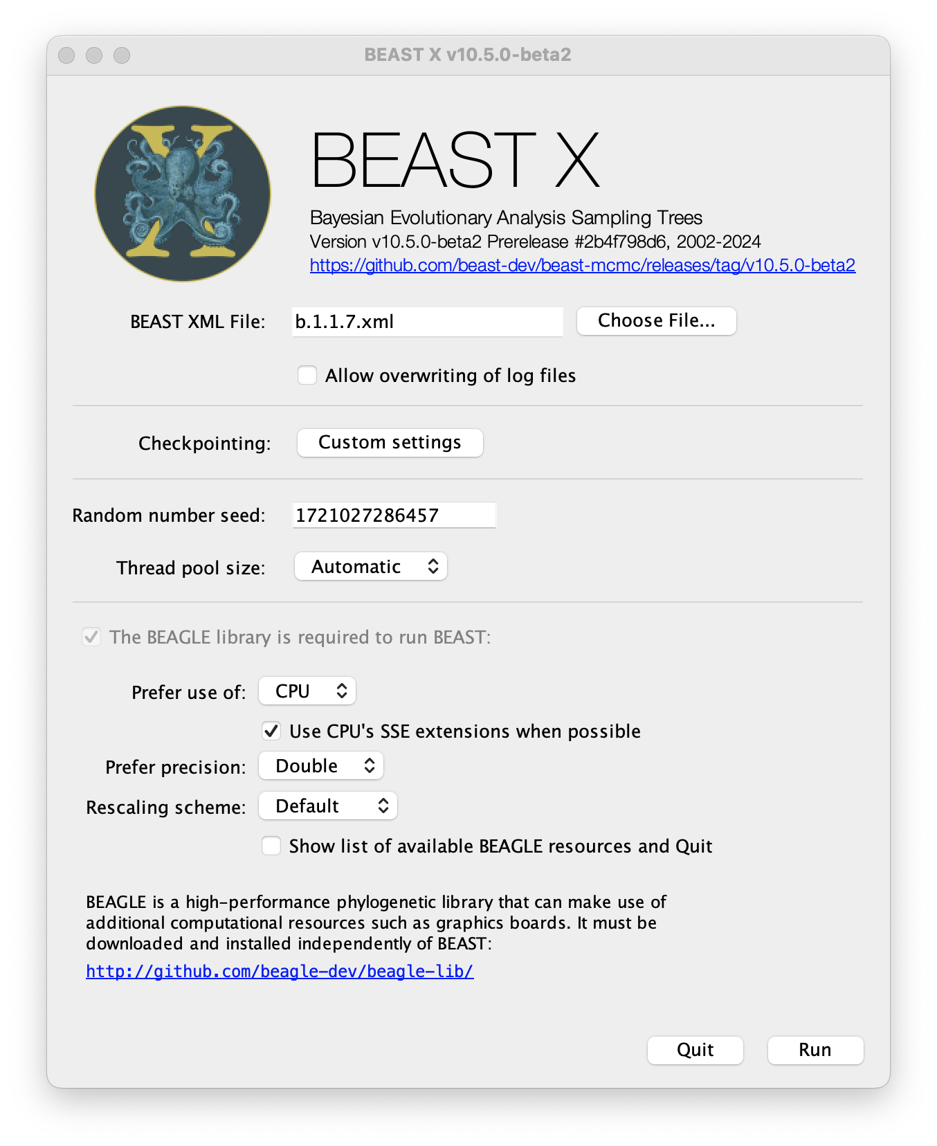
Press the Choose File... button and select the XML file you just created and press Run. The analysis will then be performed with detailed information about the progress of the run being written to the screen. When it has finished, the log file and the trees file will have been created in the same location as your XML file.
For more information about the other options in the BEAST dialog box see this page.
Analyzing the BEAST output
Select the Import Trace File... option from the File menu. Select the log file, b.1.1.7.log, that you created in the previous section. The file will load and you will be presented with a window similar to the one below.
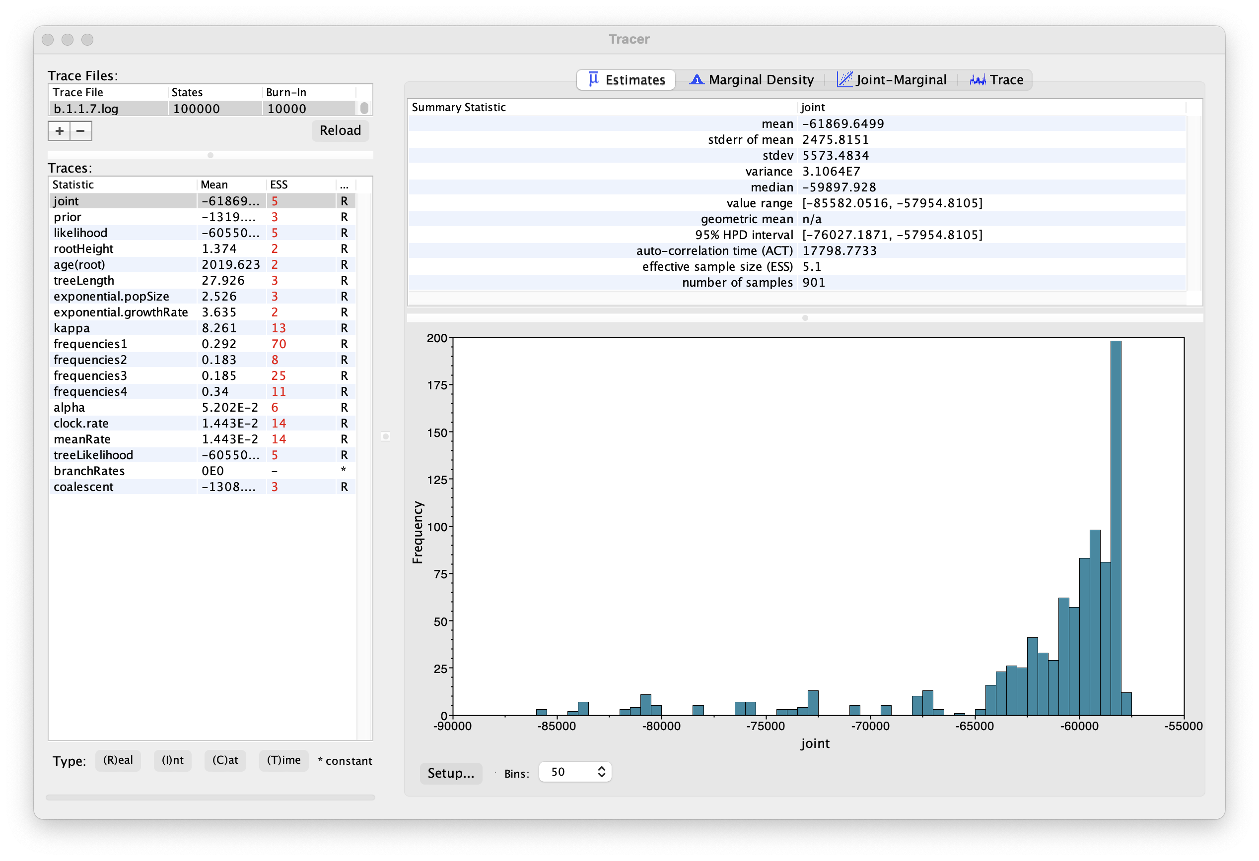
Similarly to the previous tutorial the effective sample sizes (ESSs) for all the traces are small (ESSs less 100 are highlighted in red respectively by Tracer). In the bottom right of the window is a frequency plot of the samples, which for the joint trace in the above figure, has multiple peaks.
If we select the tab on the right-hand-side labelled Trace we can view the raw trace — the sampled values against the step in the MCMC chain:
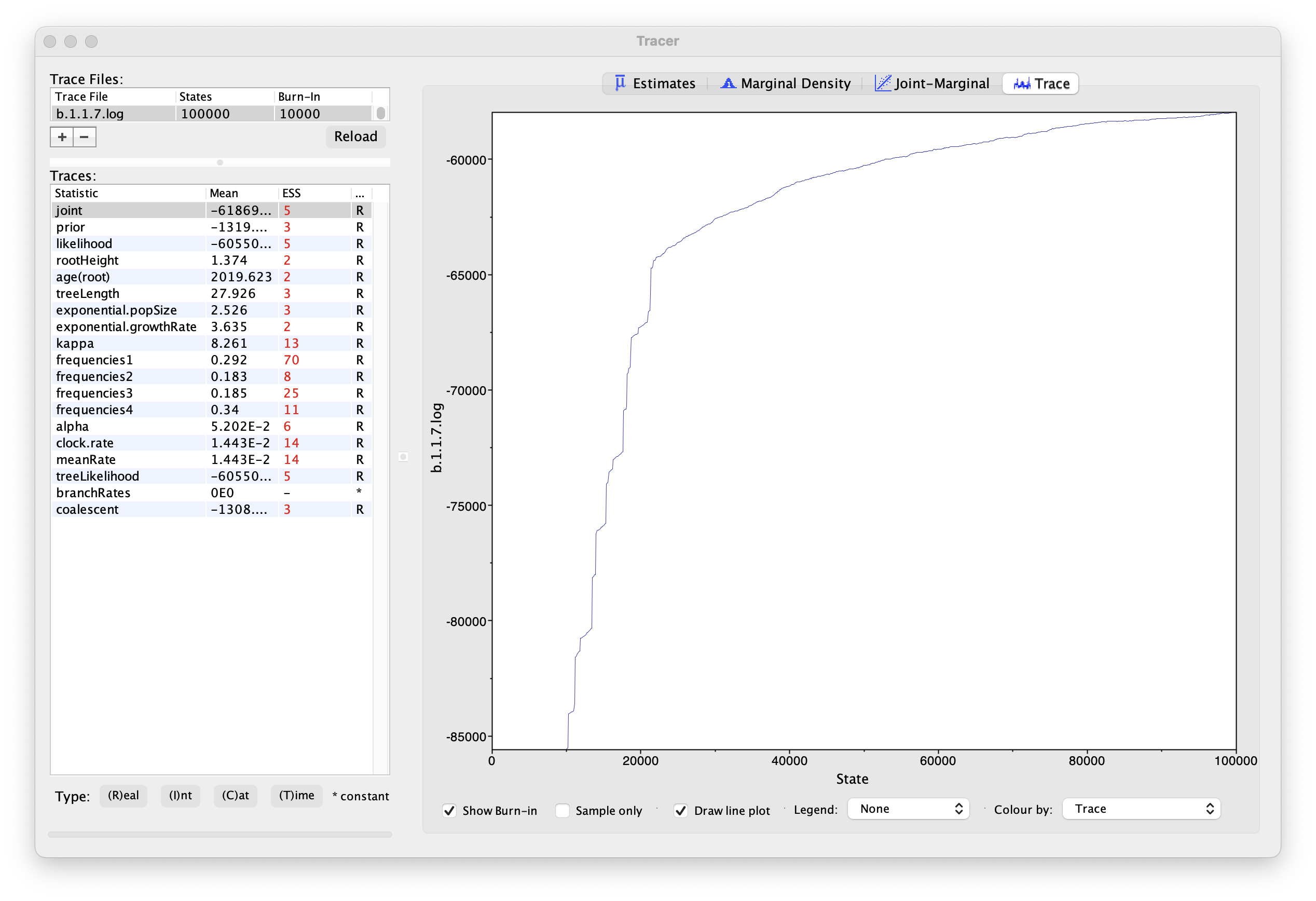
Here it is clear that the default burn-in of 10% of the chain length is inadequate (the posterior values are still increasing over the first part of the chain). It is still clear that a chain length of 100,000 was inadequate, and even increasing the burn-in will not result in a stable estimate. Looking at the ESS values (generally in the low double-digits) suggests that a much longer chain length is needed. Running much longer chains would take a considerably longer times, but we have provided the output of a run of 500 million generations that you can use for the rest of this section.
Load the new log file (b.1.1.7.log) into Tracer (you can leave the old one loaded for comparison). Click on the Trace tab and look at the raw trace plot.
Again we have chosen options that produce 1000 samples and with an ESS of > 500 for the coalescent model parameters there is little auto-correlation between the samples. There are no obvious trends in the plot which would suggest that the MCMC has not yet converged, and there are no large-scale fluctuations in the trace which would suggest poor mixing.
As we are satisfied with the behavior of the MCMC we can now move on to one of the parameters of interest: exponential growth rate for the coalescent model we chose as the tree prior. Select exponential.growthRate in the left-hand table. Now choose the density plot by selecting the tab labeled Marginal Density. This shows a plot of the marginal posterior probability density of this parameter. You should see a plot similar to this:
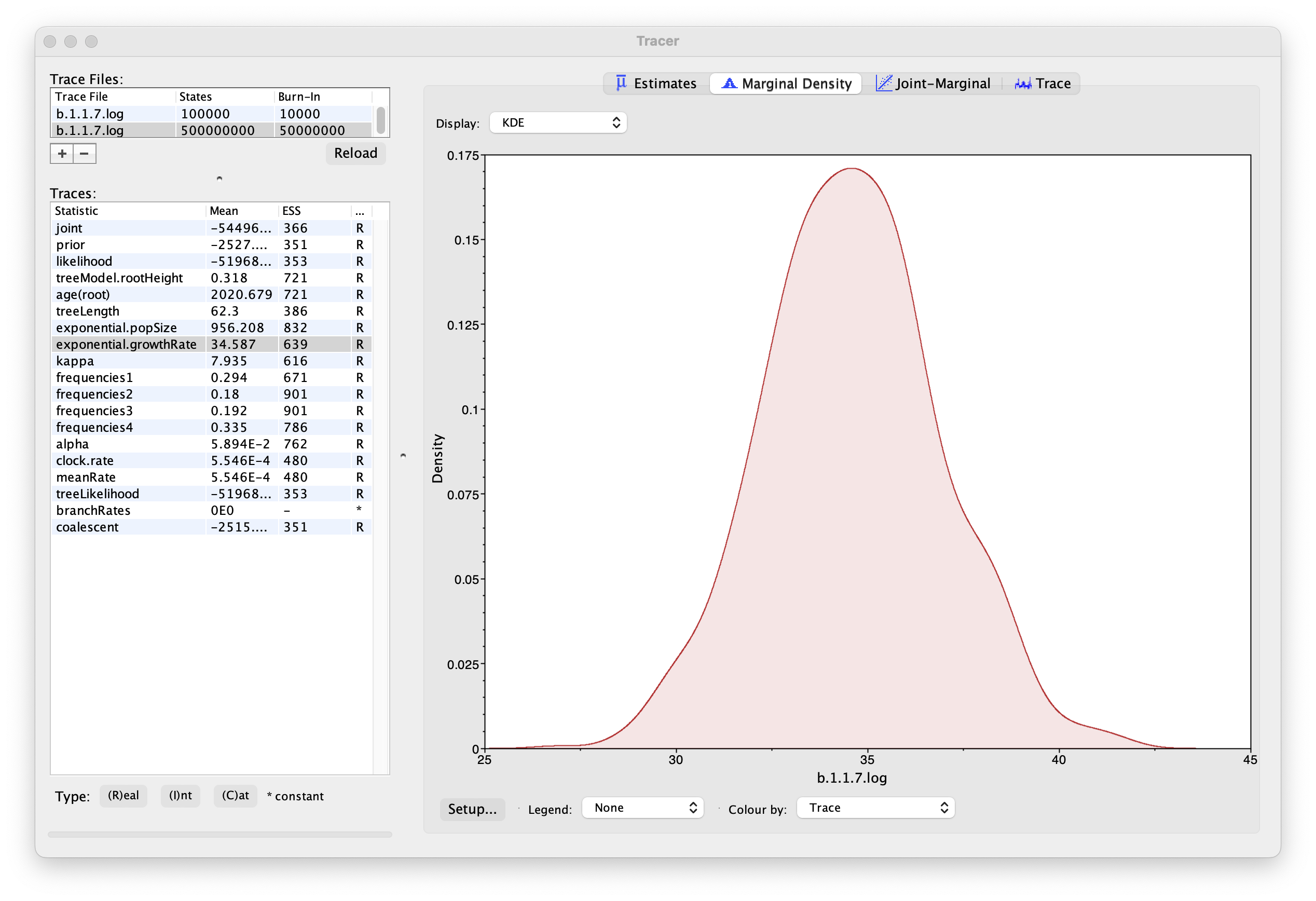
As you can see the posterior probability density is roughly bell-shaped. The default is to show the kernel density estimate (KDE) which is smoothed probability density fitted to the data. Switch the Display: option at the top to Histogram to see the unsmoothed frequency plot. There is still a lot of noise here but it is a good estimate of the distribution.
age(root) statistic provides an estimate of the time of the most recent common ancestor of the entire tree. In this case it may be a reasonable estimate of the emergence of the alpha variant in the U.K. What is the mean estimate and 95% HPDs for the date of the MRCA?You can visualize the growth estimate using the Demographic Reconstruction... option in the Analysis menu. Select this option and set up the dialog box that appears like this:
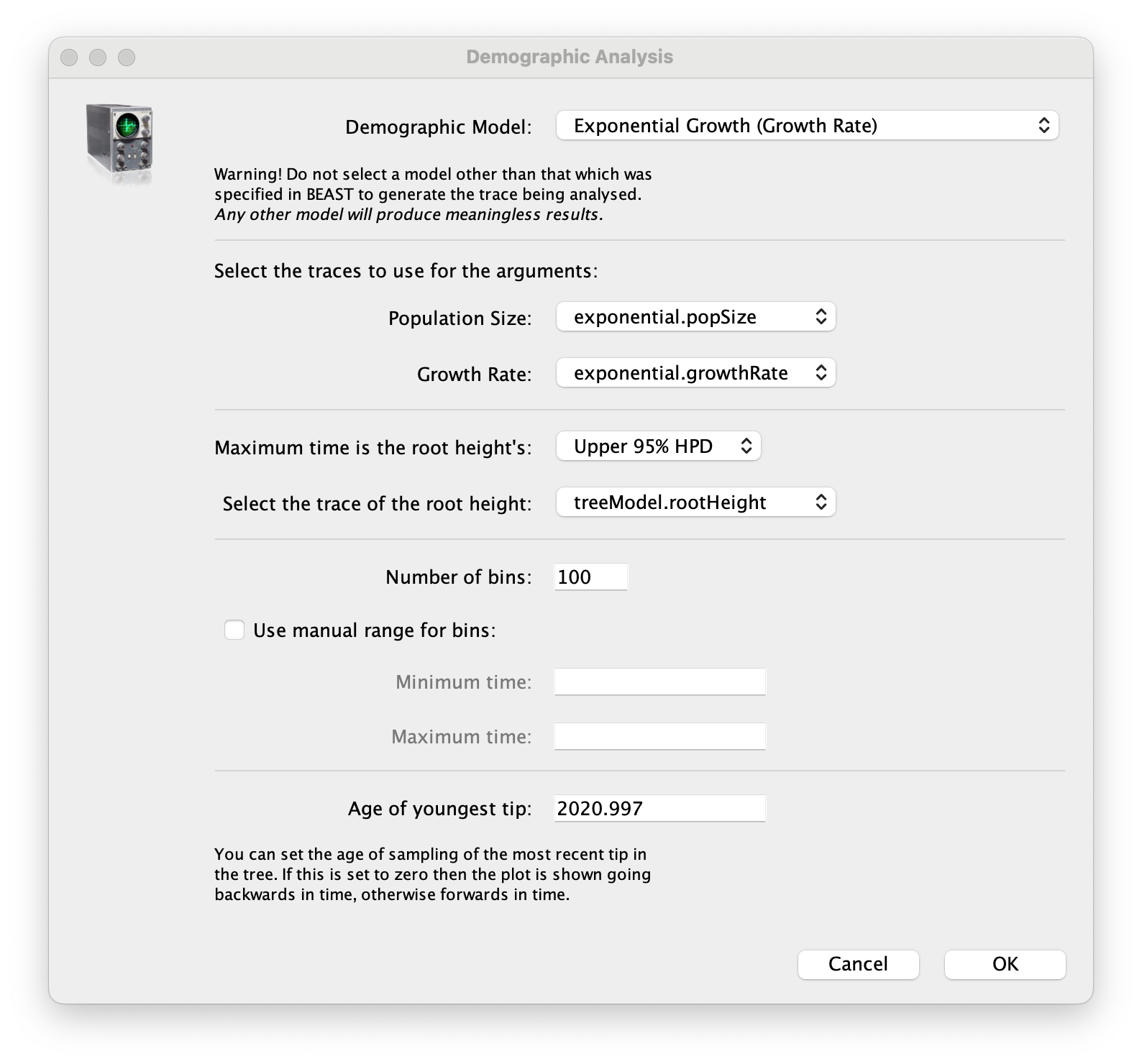
Select Demographic Model: Exponential Growth (Growth Rate) — note, you must select the tree prior you picked in BEAUti, you can’t change this here. Tracer will automatically identify the parameters of the model (exponential.popSize and exponential.growthRate). The option Maximum time is the root height's: pick the Upper 95% HPD. This means it will extend the reconstruction back to the extent of the root age credible interval. Set the Age of youngest tip: to 2020.997 (the date of the most recently sampled virus). Then press OK and this window will appear:
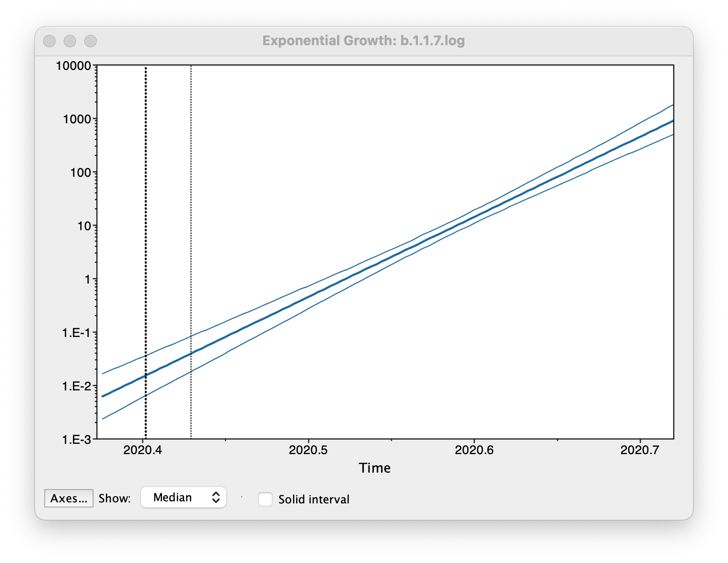
This shows the exponential growth line for the median growth rate and the 95% HPD intervals for this growth as a solid area. It is on a log scale so is a straight line. You can play with the axis settings using the Axes... button. The dotted vertical lines represent the 95% HPD for the date of the root of the tree.
An alternative way of assessing viral population growth would be through the doubling time estimate. This can be obtained based on the growth rate (how would you get this?), or it can be estimated through a coalescent growth model with a doubling time parameterisation (cfr. above).
Given the current run, how does the estimate compare to a doubling time estimate based on the spike gene target failure PCR method for Oregon, U.S., of 9.54 (Smith et al., 2022) for example?
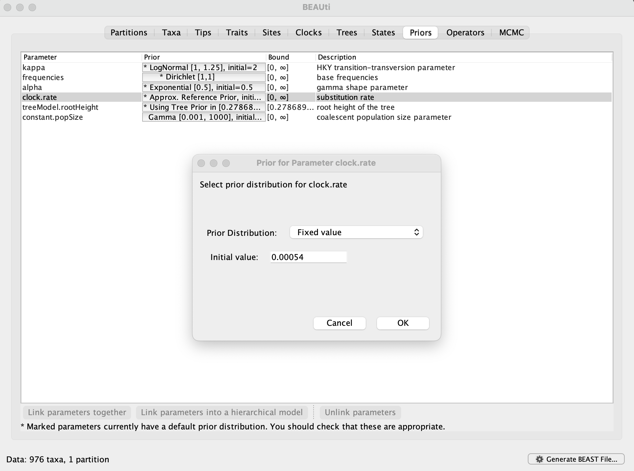
In order to compare the expansion of alpha with another SARS-CoV-2 variant in the U.K., a data set encompassing 1,000 genomes for omicron BA.1 has been made available. This is a subset of the largest transmission lineage of omicron BA.1 identified in the U.K. (Tsui et al, 2023). The subset was obtained by sampling as evenly as possible over the time period between 27 November 2021 and 25 December 2021. This time period is too short for the genome data to contain adequate temporal signal (which you can examine using TempEst). Therefore, we will fix the rate of 0.00054 substitutions per site per year, which is the posterior mean for the rate in the alpha analyses. This can be set in the Priorspanel, by selecting Fixed valueand entering 0.00054:
For this data set, we will use a serial interval distribution mean of 3 and standard deviation of 1 day (Park et al., 2023) to calculate \(R_0\). Long runs have been provided for both the growth rate and doubling time parameterisations. What are the mean estimates for \(R_0\) and the doubling time? Note that when parameterising the exponential model using the doubling time, the doubling time is in years. However, when the doubling time is calculated based on the growth rate in the analyses that parameterise with the growth rate, the doubling time is in days. How do the \(R_0\) and doubling time values compare to estimates of \(R_t = 2.1\) for South Africa (Khan et al., 2022) and a doubling time of 4.28 days for Oregon, U.S. (Smith et al., 2022)?
EXERCISE 2: reconstructing H3N2 epidemic dynamics in the New York state.
In this tutorial, we will reconstruct a Bayesian skygrid of human influenza A, H3N2 subtype, over three northern hemisphere epidemic seasons. The data set contains 165 Hemagglutinin gene sequences, and as the SARS-CoV-2 data sets, it takes more time to run in BEAST than available during a practical session. Therefore, this tutorial will discuss how to set up this analysis and how to summarize the results based on runs that have already been performed.
Running BEAUti
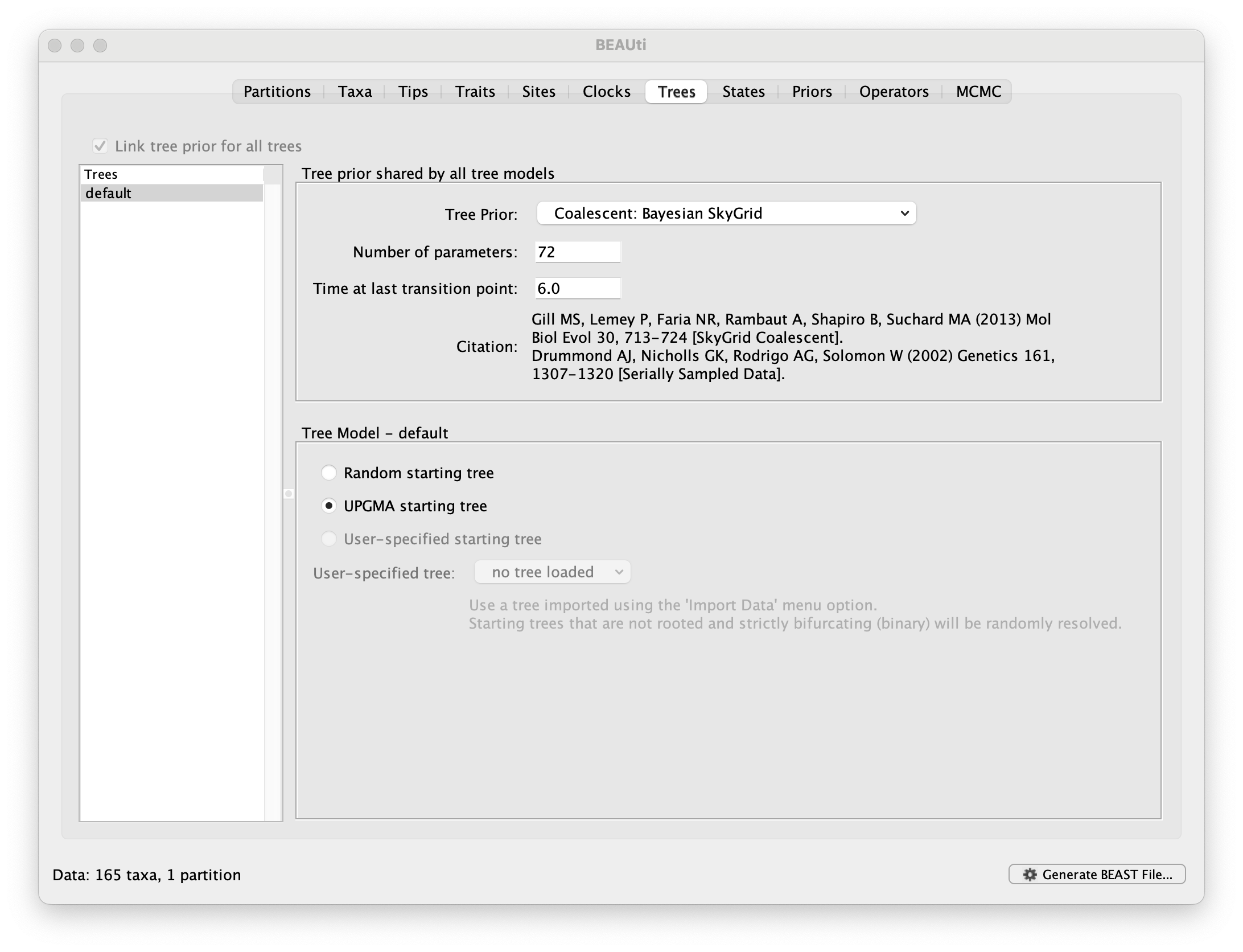
Run BEAUti, load the nexus file (NewYork.HA.2000-2003.nex) and set the Tips panel’s Parse Dates to the last numerical field in the sequence names as previously, but now with an underscore _ prefix and Parse as a number. Set the same evolutionary model (including gamma distributed rate variation) and clock model as in the previous exercise. In the Trees tab, select a Coalescent: Bayesian SkyGrid as the Tree Prior. We will construct a grid of 72 intervals over 6 years (Time at last point: 6) before the most recent sampling date (2003.98 in our case, so going back to about 1998) thus estimating 12 population sizes per year. The panel should look like this:
At this point we would usually generate the BEAST XML file, load it into BEAST and run it. However, this data set, while smaller than the SARS-CoV-2 data sets, is still relatively computationally intensive so rather than waiting around for it to finish, you can go straight on and analyse some results files that have already been run.
Analyzing the BEAST output
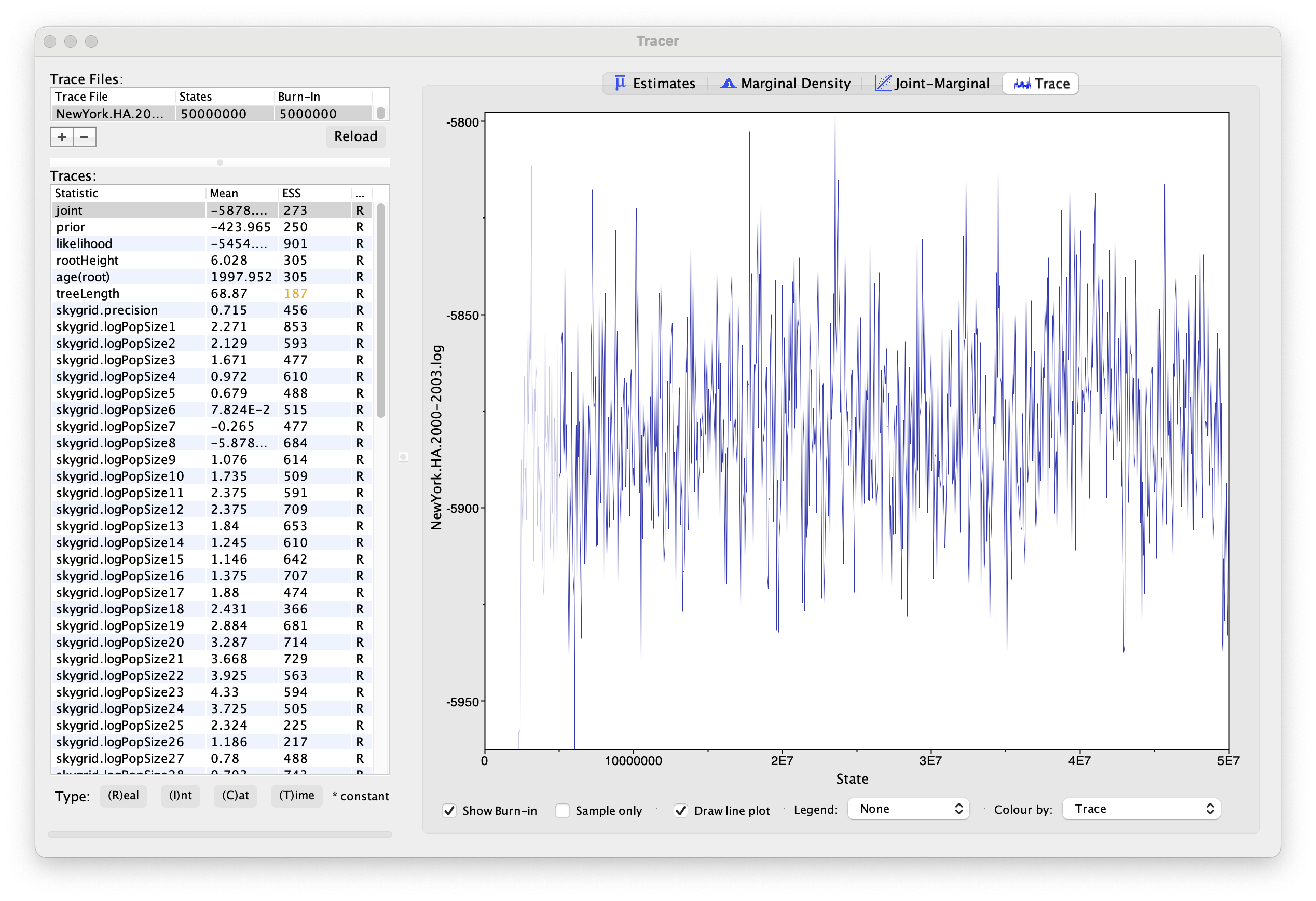
Using Tracer, we can analyze the run based on the output files provided (load the file called NewYork.HA.2000-2003.log). This has been run with a chain length of 50,000,000 generations sampling every 50,000 steps so a total of 1,000 samples:
To reconstruct the Bayesian skygrid plot, select SkyGrid reconstruction... under the Analysis menu. The following window should appear:
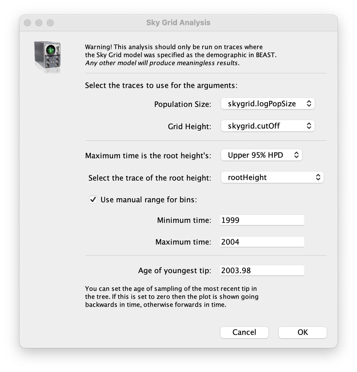
Set the manual bin range from 1999 to 2004 and specify 2003.98 as the Age of the youngest tip at the bottom. Press OK and after some time, the following Bayesian skyGrid reconstruction should appear (with solid interval selected):
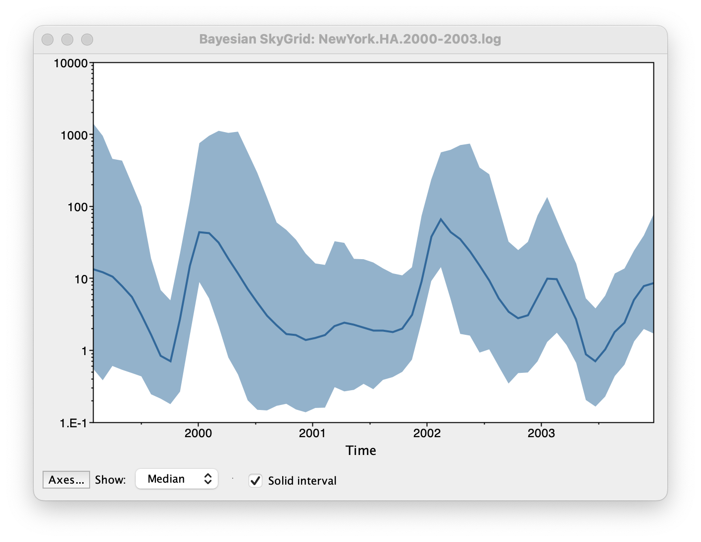
By default the y-axis is in a log scale. Press the Axes button and turn off Log axis for the Y axis. You will also need to set the Manual range because the upper HPD bounds will be very large. Set this to 0 to 100 and you get the following:
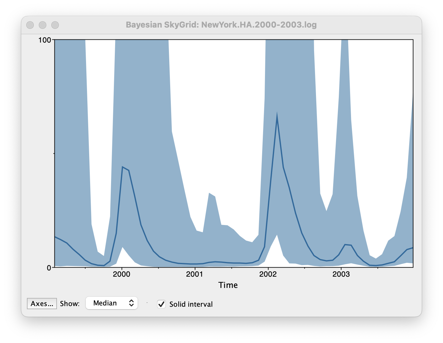
This clearly shows the seasonal peaks but the uncertainty represented by the credible intervale is very large.
Some Questions
References
- Drummond AJ, Rambaut A (2007) BEAST: Bayesian evolutionary analysis by sampling trees. BMC Evolutionary Biology 7: 214.
- Drummond AJ, Ho SYW, Phillips MJ & Rambaut A (2006) PLoS Biology 4, e88.
- Drummond AJ, Rambaut A & Shapiro B and Pybus OG (2005) Mol Biol Evol 22, 1185-1192.
- Drummond AJ, Nicholls GK, Rodrigo AG & Solomon W (2002) Genetics 161, 1307-1320.
- Ferreira, M. A. R. and M. A. Suchard. 2008. Bayesian analysis of elapsed times in continuous-time Markov chains. Can J Statistics, 36: 355–368. doi: 10.1002/cjs.5550360302
- Gill MS, Lemey P, Faria NR, Rambaut A, Shapiro B, and Suchard MA (2013) Improving Bayesian population dynamics inference: a coalescent-based model for multiple loci. Mol Biol Evol 30, 713-724.
- Hill V, Du Plessis L, Peacock TP, Aggarwal D, Colquhoun R, Carabelli AM, Ellaby N, Gallagher E, Groves N, Jackson B, McCrone JT, O’Toole Á, Price A, Sanderson T, Scher E, Southgate J, Volz E, Barclay WS, Barrett JC, Chand M, Connor T, Goodfellow I, Gupta RK, Harrison EM, Loman N, Myers R, Robertson DL, Pybus OG, Rambaut A. The origins and molecular evolution of SARS-CoV-2 lineage B.1.1.7 in the UK. Virus Evol. 2022 Aug 26;8(2):veac080. doi: 10.1093/ve/veac080. Erratum in: Virus Evol. 2022 Dec 30;8(2):veac119. PMID: 36533153; PMCID: PMC9752794.
- Khan MA, Atangana A. Mathematical modeling and analysis of COVID‐19: a study of new variant Omicron. Physica A. 2022. https://doi.org/10. 1016/j.physa.2022.127452.
- Minin VN, Bloomquist EW and Suchard MA (2008) Smooth Skyride through a Rough Skyline: Bayesian Coalescent-Based Inference of Population Dynamics. Molecular Biology and Evolution 25:1459-1471; doi:10.1093/molbev/msn090.
- Park SW, Sun K, Abbott S, Sender R, Bar-On YM, Weitz JS, Funk S, Grenfell BT, Backer JA, Wallinga J, Viboud C, Dushoff J. Inferring the differences in incubation-period and generation-interval distributions of the Delta and Omicron variants of SARS-CoV-2. Proc Natl Acad Sci U S A. 2023 May 30;120(22):e2221887120. doi: 10.1073/pnas.2221887120. Epub 2023 May 22. PMID: 37216529; PMCID: PMC10235974.
- Rambaut A, Pybus OG, Nelson MI, Viboud C, Taubenberger JK, Holmes EC (2008) The genomic and epidemiological dynamics of human influenza A virus. Nature, 453: 615-9.
- Smith, B. F., Graven, P. F., Yang, D. Y., Downs, S. M., Hansel, D. E., Fan, G., & Qin, X. (2022). Using Spike Gene Target Failure to Estimate Growth Rate of the Alpha and Omicron Variants of SARS-CoV-2. Journal of Clinical Microbiology, 60(4). https://doi.org/10.1128/jcm.02573-21.
- Joseph L.-H. Tsui et al. (2023). Genomic assessment of invasion dynamics of SARS-CoV-2 Omicron BA.1.Science381,336-343(2023).DOI:10.1126/science.adg6605.
- Volz, E., Mishra, S., Chand, M. et al. Assessing transmissibility of SARS-CoV-2 lineage B.1.1.7 in England. Nature 593, 266–269 (2021). https://doi.org/10.1038/s41586-021-03470-x.
Help and documentation
The BEAST website: http://beast.community
Tutorials: http://beast.community/tutorials
Frequently asked questions: http://beast.community/faq