Analysing BEAST output using Tracer
This document provides a step-by-step tutorial to analysing the output of BEAST in a GUI application called Tracer 1.7.
Running Tracer
The exact instructions for running Tracer differs depending on which computer you are using. Please see the README text file that was distributed with the version you downloaded. Once running, Tracer will look similar irrespective of which computer system it is running on. For this tutorial, the Mac OS X version will be shown but the Linux and Windows versions will have exactly the same layout and functionality.
Note that loading extremely large output files into Tracer may cause it to become unresponsive.
Should that be the case, we suggest to allocate more memory to Tracer, which can be done by running Tracer from command line (e.g. using the tracer.jar in the lib folder of the Tracer download).
For example, to allocate 4Gb of memory to Tracer, run the following from command line:
java -Xmx4096m -jar tracer.jar
Data set information
For this tutorial, if you have it available, you can use the log file that you created in the first tutorial.
Here, we use Tracer 1.7 to infer the spatial dispersal and cross-species dynamics of rabies virus (RABV) in North American bat populations. The data set consists of 372 nucleoprotein gene sequences (nucleotide positions: 594–1353) and comprises a total of 17 bat species sampled between 1997 and 2006 across 14 states in the United States (Streicker et al., Science, 2010, 329, 676-679). Following Faria et al. (Phil. Trans. Roy. Soc. B, 2013), two additional species that had been excluded from the original analysis owing to a limited amount of available sequences, Myotis austroriparius (Ma) and Parastrellus hesperus (Ph), are also included here. We also include a viral sequence with an unknown sampling date (accession no. TX5275, sampled in Texas from Lasiurus borealis). A uniform prior specification for the age of TX5275 adequately is used in our inference, based on the assumption that its sampling time is bounded by the sampling time distribution of the data set, implying that it is sampled between 1997.5 and 2005.5. We estimate RABV ancestral locations and host-jumping history using a Bayesian discrete phylogeographic approach with BSSVS (Lemet et al., 2009), while simultaneously estimating effective population sizes over time through a Bayesian skygrid coalescent model (Gill et al., 2012).
The main Tracer panel
To load the BEAST log file(s), select the Open option from the File menu or drag and drop the log file into the Tracer window. The file will load and you will be presented with a window similar to the one below. Remember that BEAST is a stochastic program so the actual numbers will not be exactly the same.
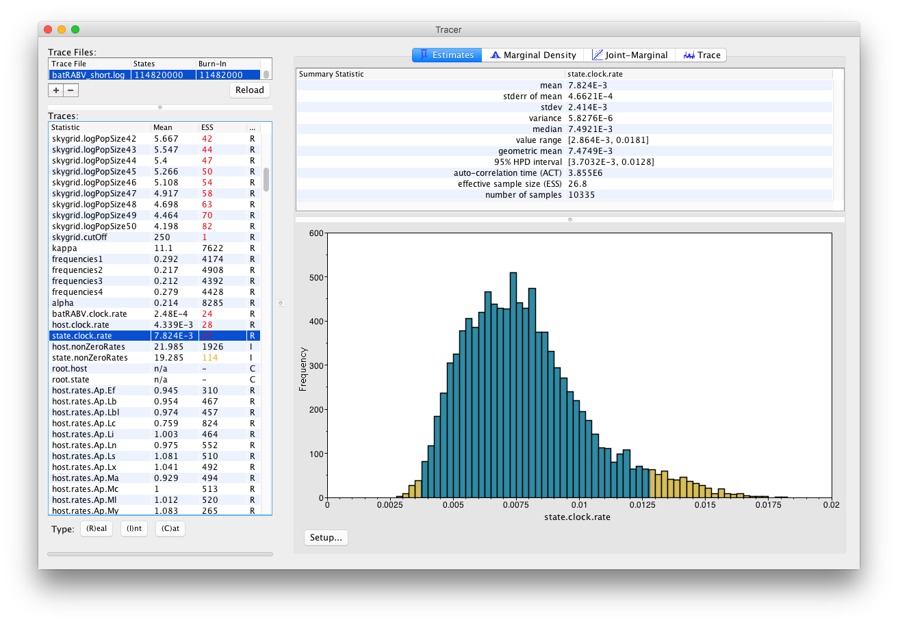
On the left hand side is the name of the log file loaded and the traces that it contains. There are traces for the posterior, prior, likelihood, and all the integer, categorical and continuous parameters that are being estimated. Selecting a trace on the left brings up analyses for this trace on the right hand side depending on the tab that is selected and the parameter type (Real/Integer/Categorical). In the figure above, the state.clock.rate trace is selected and various statistics of this trace is shown under the Estimates tab.
Note that the Effective Sample Sizes(ESSs) for many of the traces are small (ESSs less than 100 are highlighted in red by Tracer). This indicates that the current analysis did not yet yield a sufficient number of independent samples from the posterior distribution for that parameter. A low ESS means that the trace contained a lot of correlated samples and thus may not represent the posterior distribution well. In the bottom right of the window is a frequency plot of the samples.
In the top right of the window is a table of calculated statistics for the selected trace. The statistics and their meaning are described in the table below.
Mean- The mean value of the sampled trace across the chain (excluding the burn-in).
Stdev- The standard deviation of the mean. This takes into account the effective sample size so a small ESS will give a large Stdev.
Median- The median value of the sampled trace across the chain (excluding the burn-in).
95% HPD Lower- The lower bound of the highest posterior density (HPD) interval. The HPD is a credible set that contains 95% of the sampled values.
95% HPD Upper- The upper bound of the highest posterior density (HPD) interval. The HPD is a credible set that contains 95% of the sampled values.
Auto-Correlation Time (ACT)- The number of states in the MCMC chain that two samples have to be from each other for them to be uncorrelated. The ACT is estimated from the samples in the trace (excluding the burn-in).
Effective Sample Size (ESS)- The ESS is the number of independent samples that the trace is equivalent to. This is essentially the chain length (excluding the burn-in) divided by the ACT.
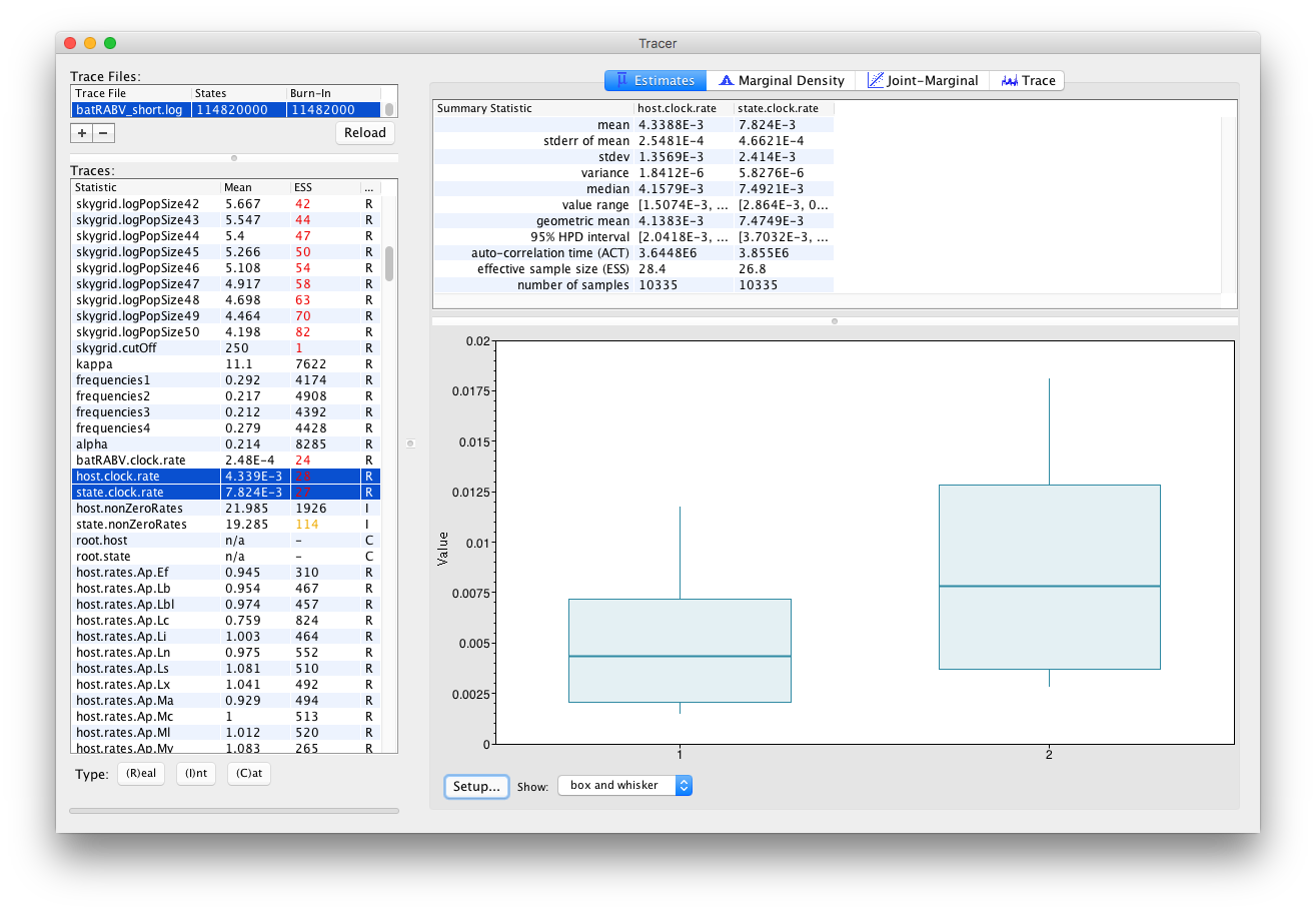
Selecting two parameters in the left column creates (by default) box and whisker plots for continuous parameters:
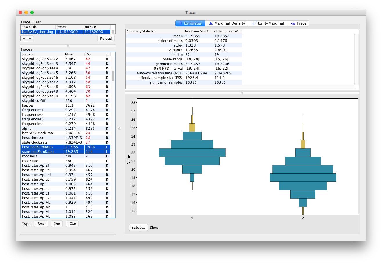
An alternative visualization is available when selecting multiple parameters of the Integer trace type:
The Trace panel
If we select the Trace (panel) we can view the raw trace, that is, the sampled values against the step in the MCMC chain:
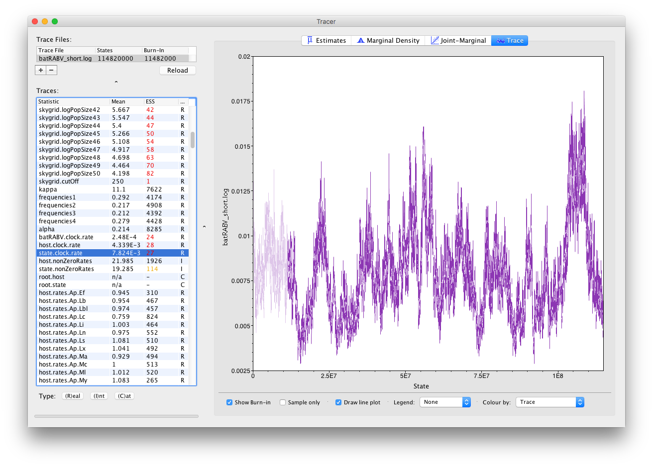
Here you can see a visual explanation of the low ESS value for the state.clock.rate parameter, with that parameter’s posterior distribution being difficult to explore. The ESS for the likelihood is about 25 so we are only getting one eighth of the amount of independent samples as actual samples. Essentially, this means we need to run the chain eight times as long to reach an ESS value of about 200. Alternatively, given that many parameters have very high ESS values (such as the kappa parameter of the HKY model), we can alter the weights on the various transition kernels to spend more time estimating the state.clock.rate parameter.
In general, substitution model parameters are fairly easy to estimate, which quickly leads to high ESS values. We can have a look at the trace of that kappa parameter to get an idea of what our trace for state.clock.rate would ideally look like (we call this plot the hairy caterpillar):
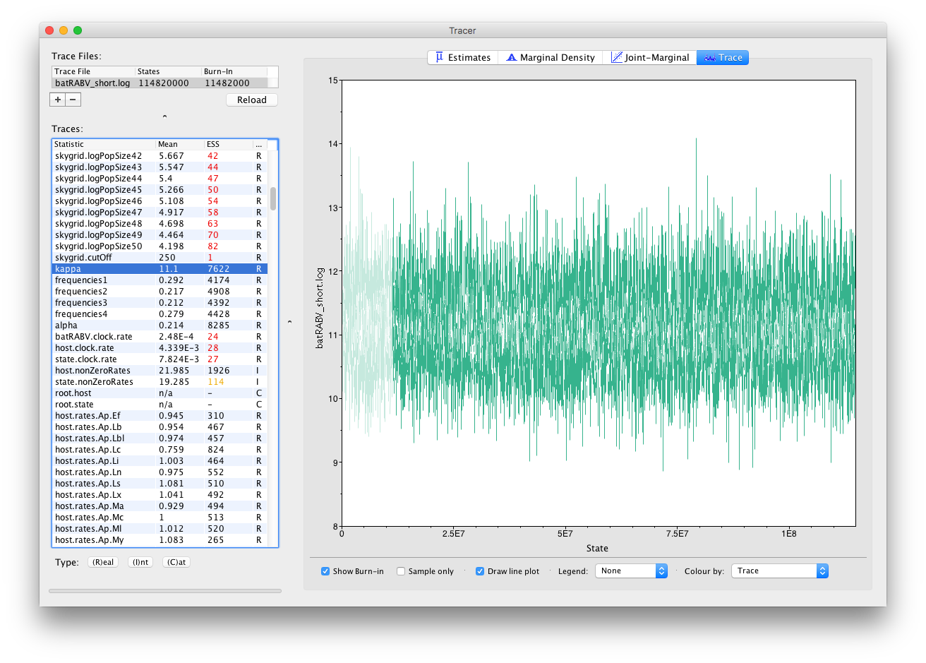
There are no obvious trends in the plot suggesting that the MCMC was still converging and there are no large-scale fluctuations in the trace suggesting poor mixing. Diagnosis of trace plots will be dealt with in a another tutorial.
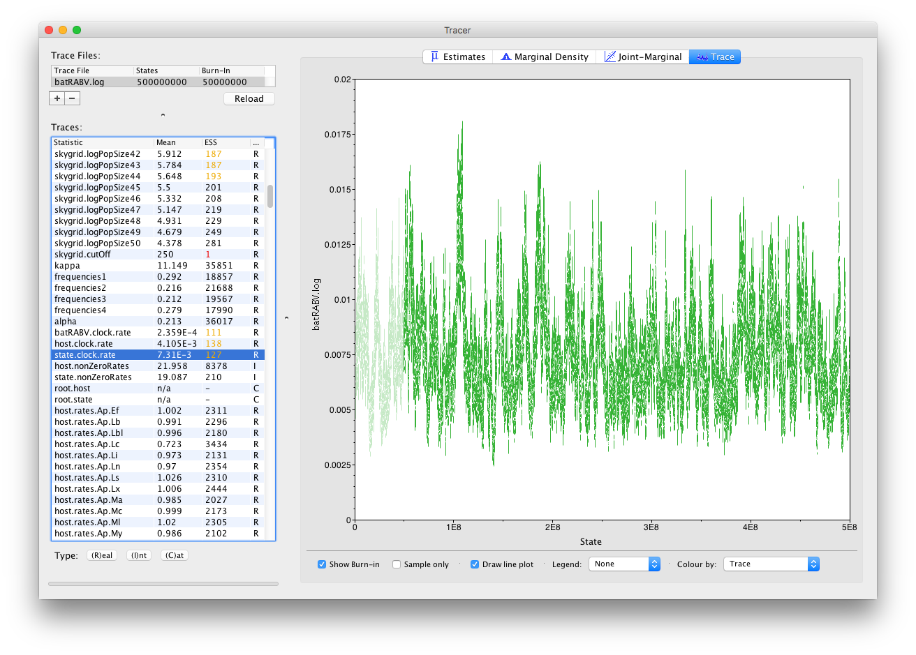
Now, let’s run our XML for about 5 times as long for a total of 500 million iterations and have a look at the state.clock.rate parameter again. This already looks much better, with its ESS value having increased by about 5, which is reflected in the trace:
It’s also straight forward to visualize the tracer for multiple parameters at the same time. Simply selecting those parameters in the left column will take care of this:
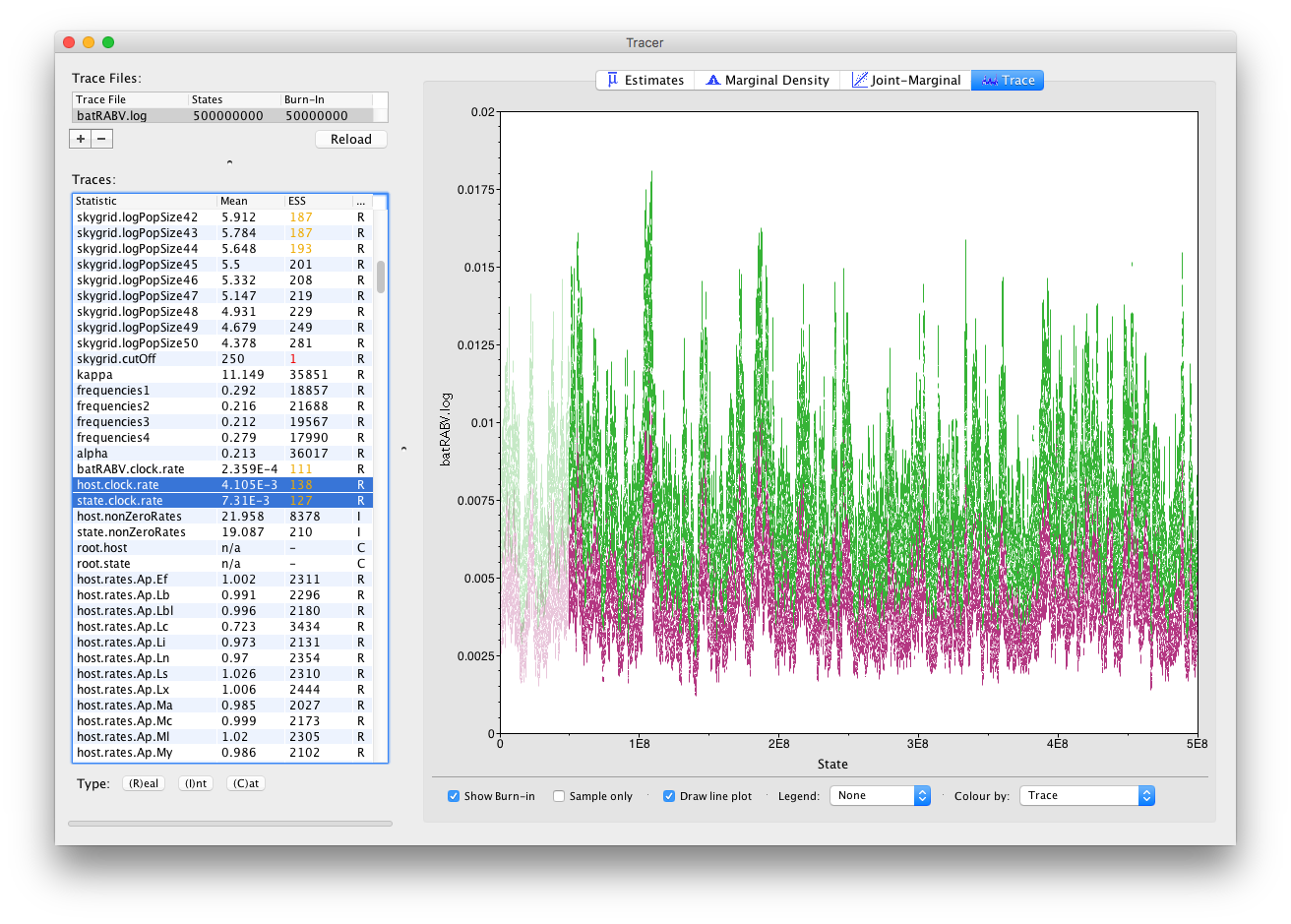
Notice how all the other parameters now also show (much) increased ESS values, such as for the population size parameters of our skygrid model. Most of those parameters have ESS values of about 200, meaning there is still auto-correlation between the samples but 200 effectively independent samples is fairly acceptable. Note that, while this analysis consists of multiple parameter types (Real/Integer/Categorical), ESS values only apply to Real (or continuous) parameters.
A separate reference page on ESS values and how to increase them is available.
The Marginal Density panel
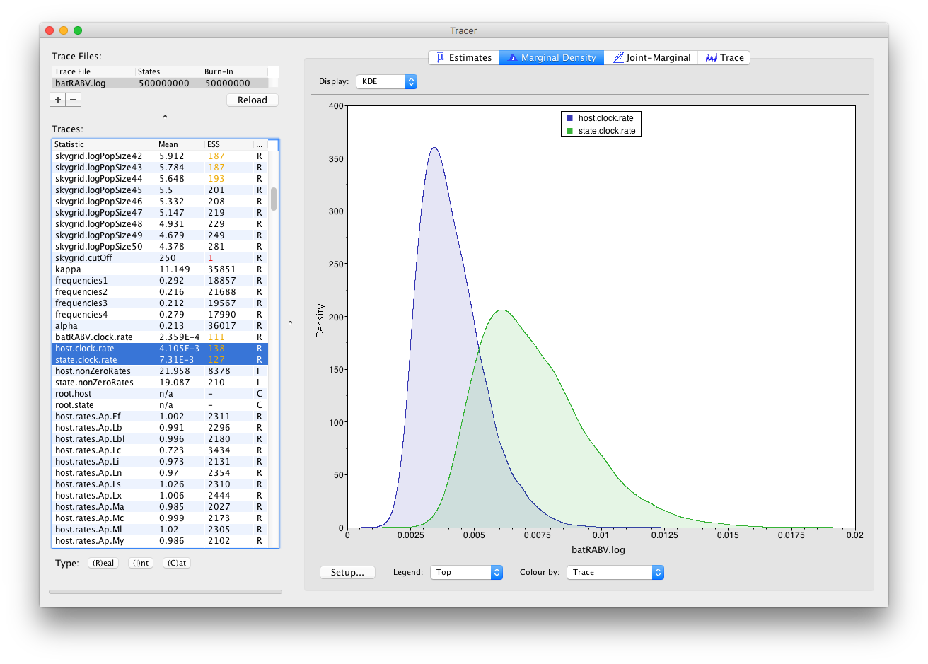
Keeping our selection of two parameters (host.clock.rate and state.clock.rate) and switching to the Marginal Density panel provides us with the following kernel density plot:
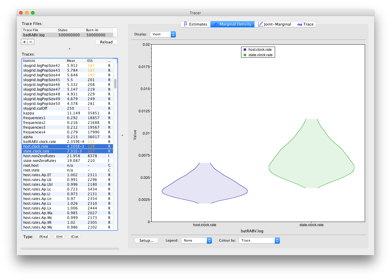
It’s convenient to switch between these kernel density plots and other visualization options, such as histograms and violin plots for continuous parameters. For example, a violin plot of our two currently selected parameters shows the following:
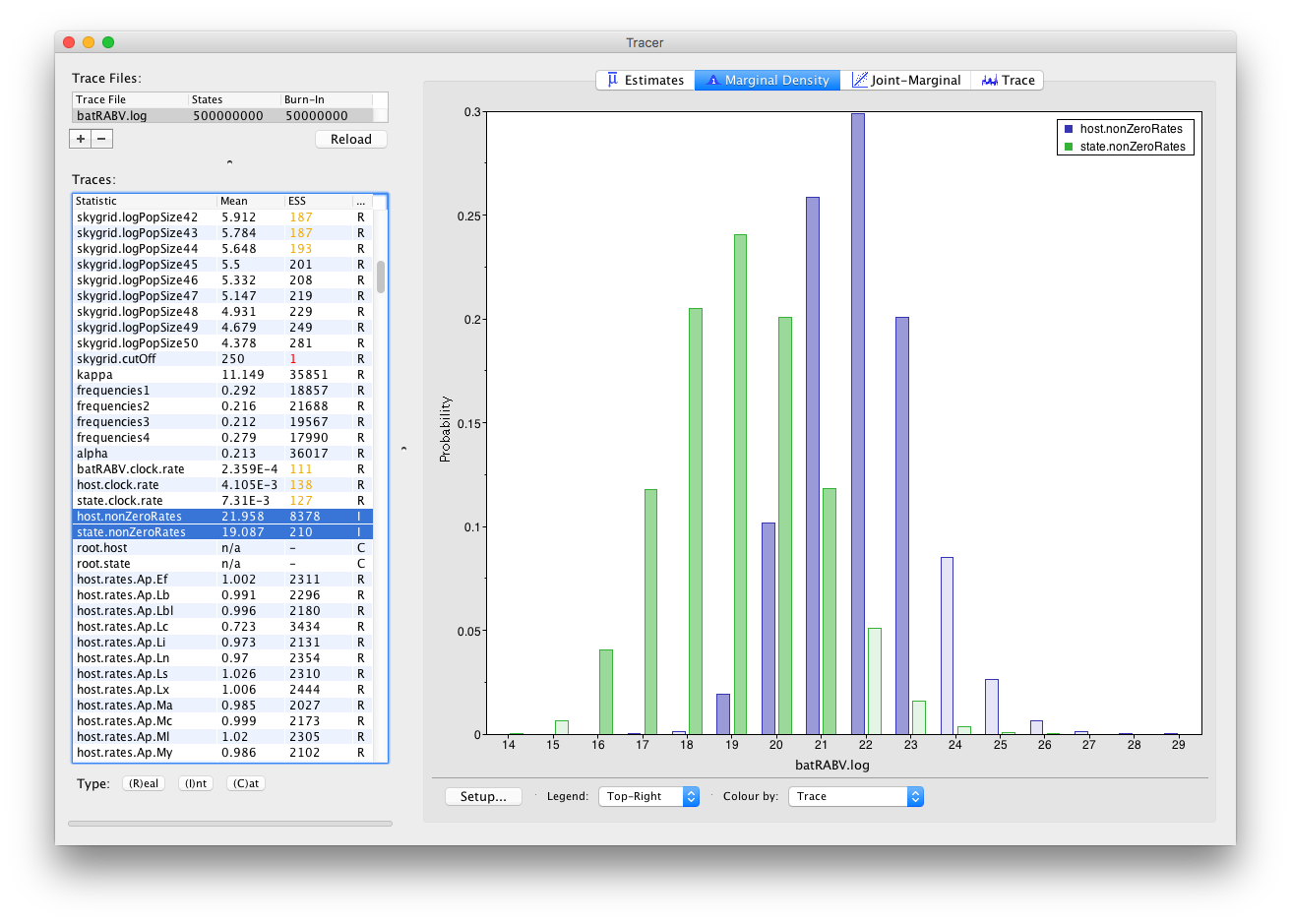
Frequency plots are used to visualize (multiple) parameters of the Integer type:
Histograms are used to visualize a parameter of the Categorical type:

The Joint-Marginal panel
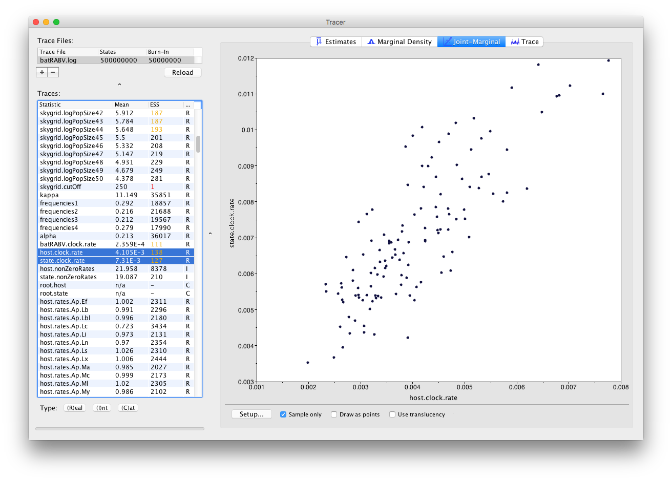
Much like the Marginal Density panel, the visualization options in the Joint-Marginal panel depend on the trace type of the selected parameter(s). Selecting two continuous (or Real) parameters leads to a classic scatter plot being shown, allowing to assess the correlation between those parameters:
When multiple continuous (or Real) parameters are selected, extensions for correlations using large correlation matrices are used (Murdoch and Chow; 1996):
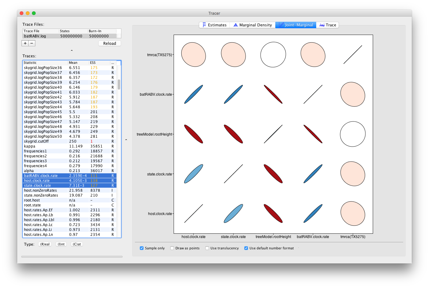
Colour gradients indicate strength and direction of the correlation, from red (strong negative) to blue (strong positive). Ellipse shapes re-enforce the strength of correlation, with no correlation appearing as a circle and perfect (anti-)correlation as a line.
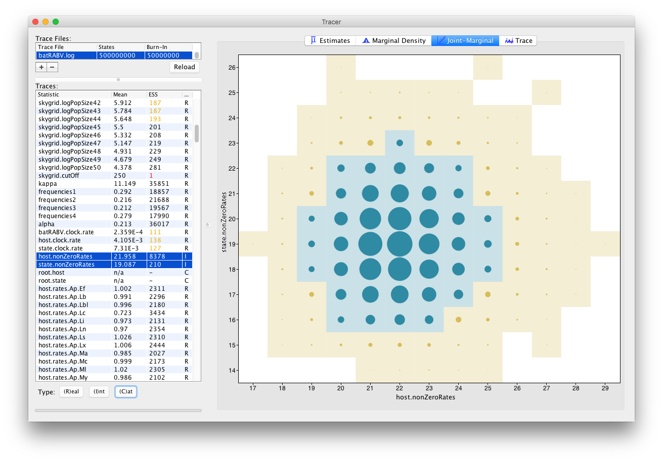
For Integer parameters, selecting exactly two parameters yields a visualization of the joint probability distribution of those two integer variables through a bubble chart:
Tracer 1.7 also allows selecting parameters of different trace types, such as one Integer and one Real parameter:
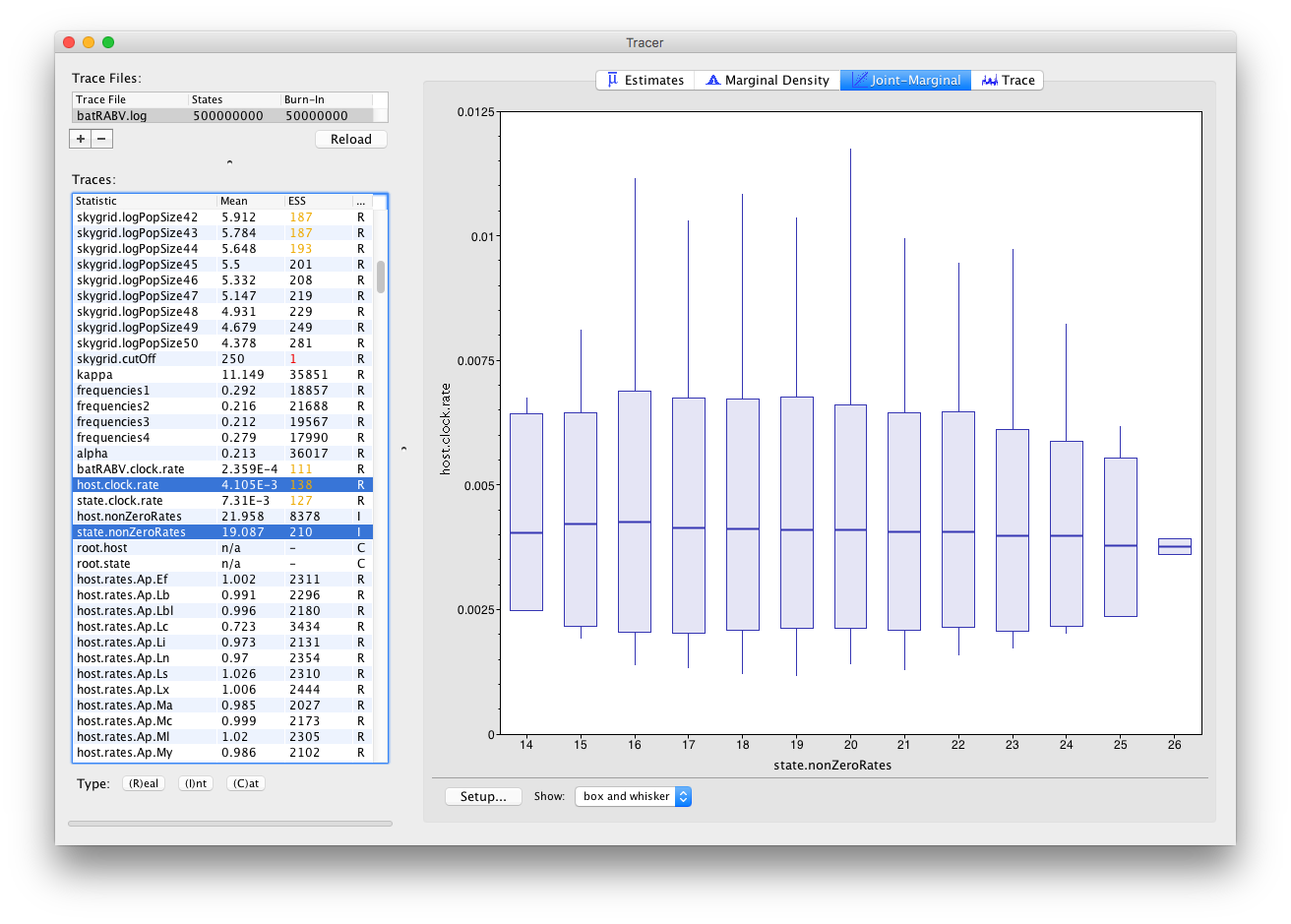
This draws one box and whisker plot for each unique value of the Integer parameter selected.
Visualizing effective population sizes over time
Tracer 1.7 provides demographic reconstruction resulting in a graphical plot, often applied to reconstruct epidemic dynamics. Available models are constant size, exponential and logistic growth (Drummond et al., 2002), and the non-parametric Bayesian skyline (Drummond et al., 2005; Heled and Drummond, 2008), skyride (Minin et al., 2008) and skygrid (Gill et al., 2012). Note that a separate page is available on the various possible tree priors in BEAST.
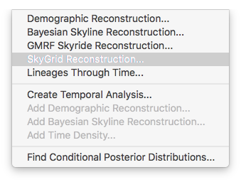
For the data analysis in this tutorial, the non-parameter skygrid coalescent model (Gill et al., 2012) was used and we show here how to perform a demographic reconstruction. In the Tracer menu bar, select Analysis which will show the following options:
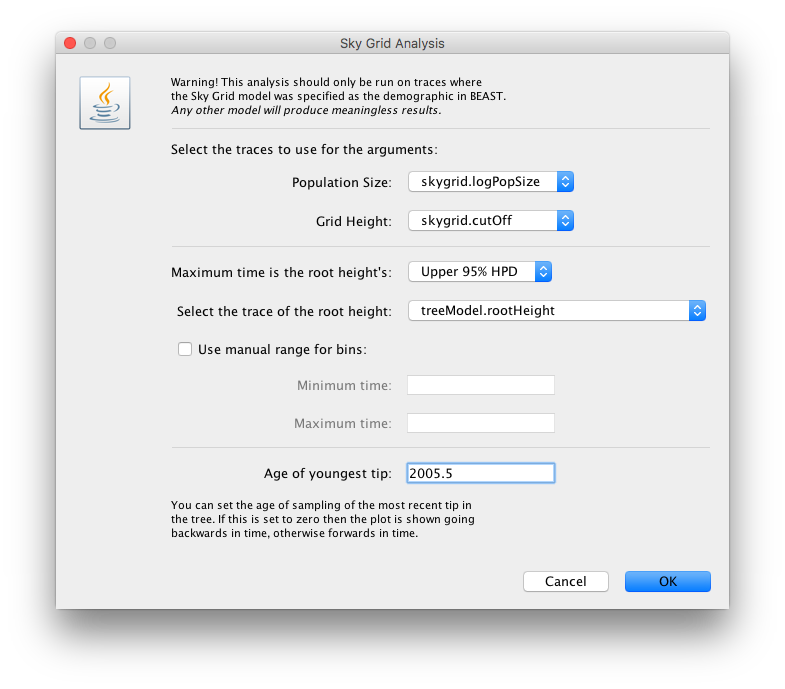
The next window allows setting various options, but typically only the ‘Age of the youngest tip’ needs to be provided:
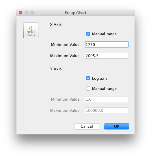
For this data set, we advise to manually set the range of the X axis in the graphical plot (which you can for any plot in Tracer 1.7):
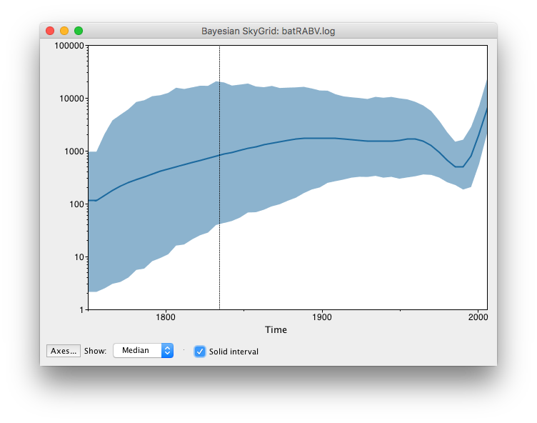
These steps allow Tracer to reconstruct the demographic history of RABV by drawing the effective population sizes over time. RABV has successfully established itself in North American bat species, with its effective population size rising steadily throughout recent centuries. Following a rapid decline at the end of last century, we observe a recent sharp increase in size.
Analysing BEAST output using TreeTracer
References
Streicker, D., Turmelle, A., Vonhof, M., Kuzmin, I., McCracken, G. F., and Rupprecht, C. (2010). Host phylogeny constrains cross-species emergence and establishment of rabies virus in bats. Science, 329, 676–679.
Faria, N., Suchard, M., Rambaut, A., Streicker, D., and Lemey, P. (2013). Simultaneously reconstructing viral cross-species transmission history and identifying the underlying constraint. Phil. Trans. R. Soc. London B, Biol. Sci., 368, 20120196.
Lemey, P., Rambaut, A., Drummond, A., and Suchard, M. (2009). Bayesian phylogeography finds its root. PLoS Comp. Biol., 5(9), e1000520.
Gill, M.S., Lemey, P., Faria, N.R., Rambaut, A., Shapiro, B. and Suchard M.A. (2013). Improving Bayesian population dynamics inference: a coalescent-based model for multiple loci. Mol. Biol. Evol. 30:713–724.
Murdoch, D. and Chow, E. (1996). A graphical display of large correlation matrices. Am. Stat., 50, 178–180.
Drummond, A. J., Nicholls, G. K., Rodrigo, A. G., and Solomon, W. (2002). Estimating mutation parameters, population history and genealogy simultaneously from temporally spaced sequence data. Genetics, 161(3), 1307–1320.
Drummond, A. J., Rambaut, A., Shapiro, B., and Pybus, O. G. (2005). Bayesian coalescent inference of past population dynamics from molecular sequences. Mol. Biol. Evol., 22(5), 1185–1192.
Heled, J. and Drummond, A. J. (2008). Bayesian inference of population size history from multiple loci. BMC Evol. Biol., 8, 289.
Minin, V. N., Bloomquist, E. W., and Suchard, M. A. (2008). Smooth skyride through a rough skyline: Bayesian coalescent- based inference of population dynamics. Mol. Biol. Evol., 25(7), 1459–1471.