In this tutorial, we will reconstruct a Bayesian skygrid of human influenza A, H3N2 subtype, over three northern hemisphere epidemic seasons. The data set contains 165 Hemagglutinin gene sequences and can take a few hours to run so this tutorial will discuss how to set up this analysis and then how to summarize the results based on runs, already performed, that can be downloaded from this site.
Running BEAUti
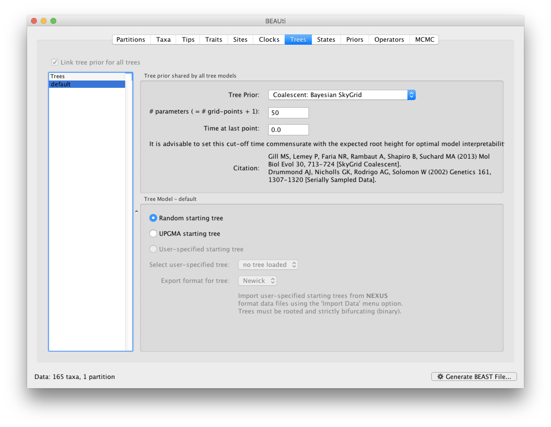
Run BEAUti, load the nexus file (NewYork.HA.2000-2003.nex) and set the Tips panel’s Parse Dates to the last numerical field in the sequence names as previously. Set the same evolutionary model (including gamma distributed rate variation) and clock model as in the previous exercise. In the Trees tab, select a Coalescent: Bayesian SkyGrid as the Tree Prior. We will construct a grid of 50 intervals over 5 years (Time at last point: 5) before the most recent sampling date (2003.98 in our case, so going back to about 1999) thus estimating 10 population sizes per year. The panel should look like this:
At this point we would usually generate the BEAST XML file, load it into BEAST and run it. However, this data set is a bit bigger than before and the model is a bit more computationally intensive so rather than waiting around for it to finish, you can go straight on an analyse some results files that have already been run.
Analyzing the BEAST output
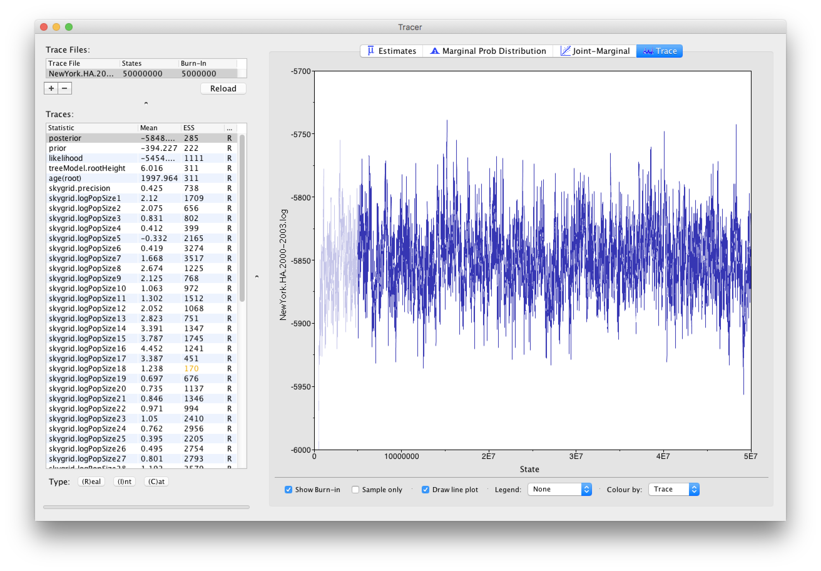
Using Tracer, we can analyze the run based on the output files provided (load the file called NewYork.HA.2000-2003.log). This has been run with a chain length of 50,000,000 sampling every 5,000 steps so a total of 10,000 samples:
To reconstruct the Bayesian skygrid plot, select SkyGrid reconstruction... under the Analysis menu. The following window should appear:
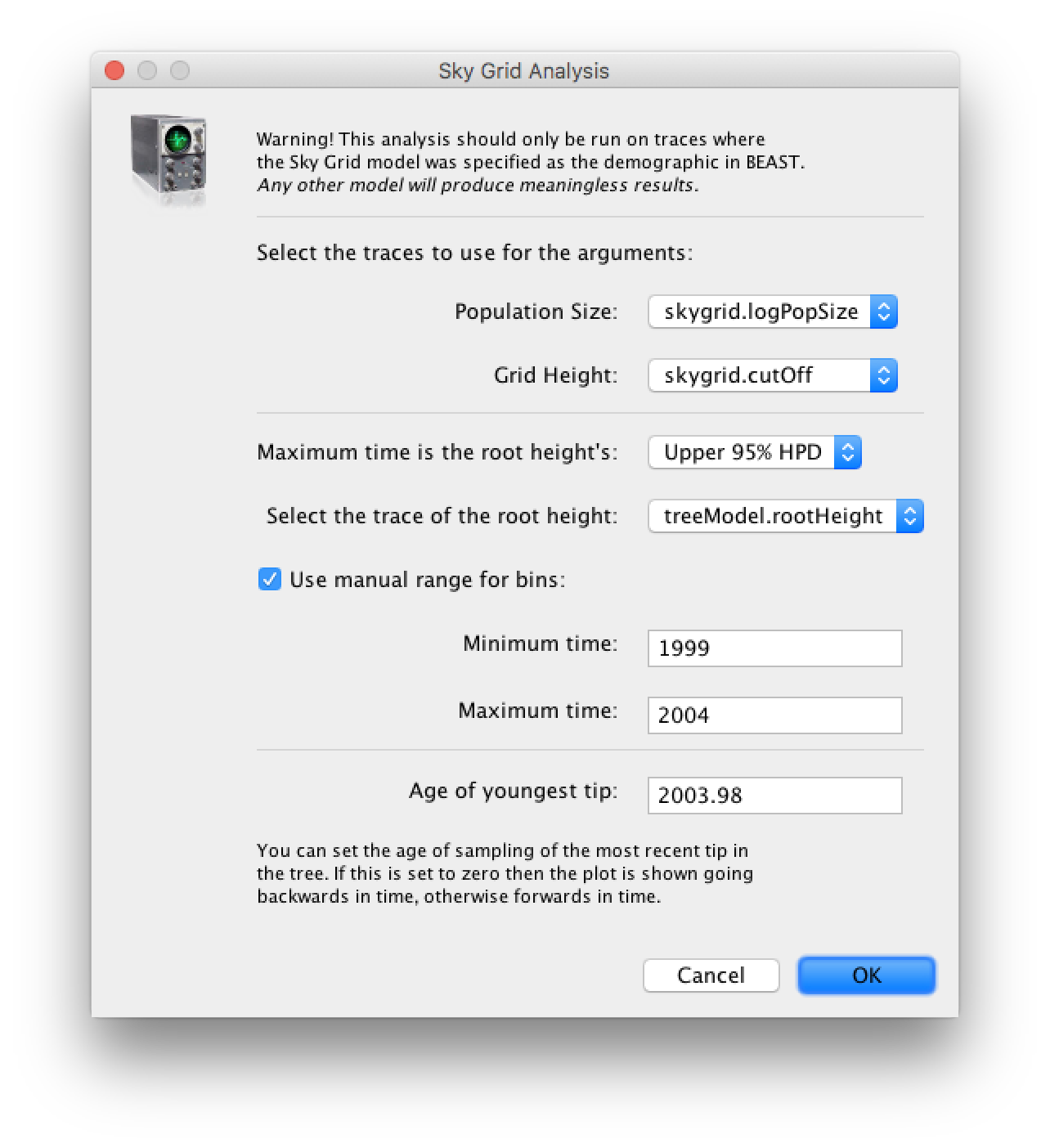
Set the manual bin range from 1999 to 2004 and specify 2003.98 as the Age of the youngest tip at the bottom. Press OK and after some time, the following Bayesian skyGrid reconstruction should appear (with solid interval selected):
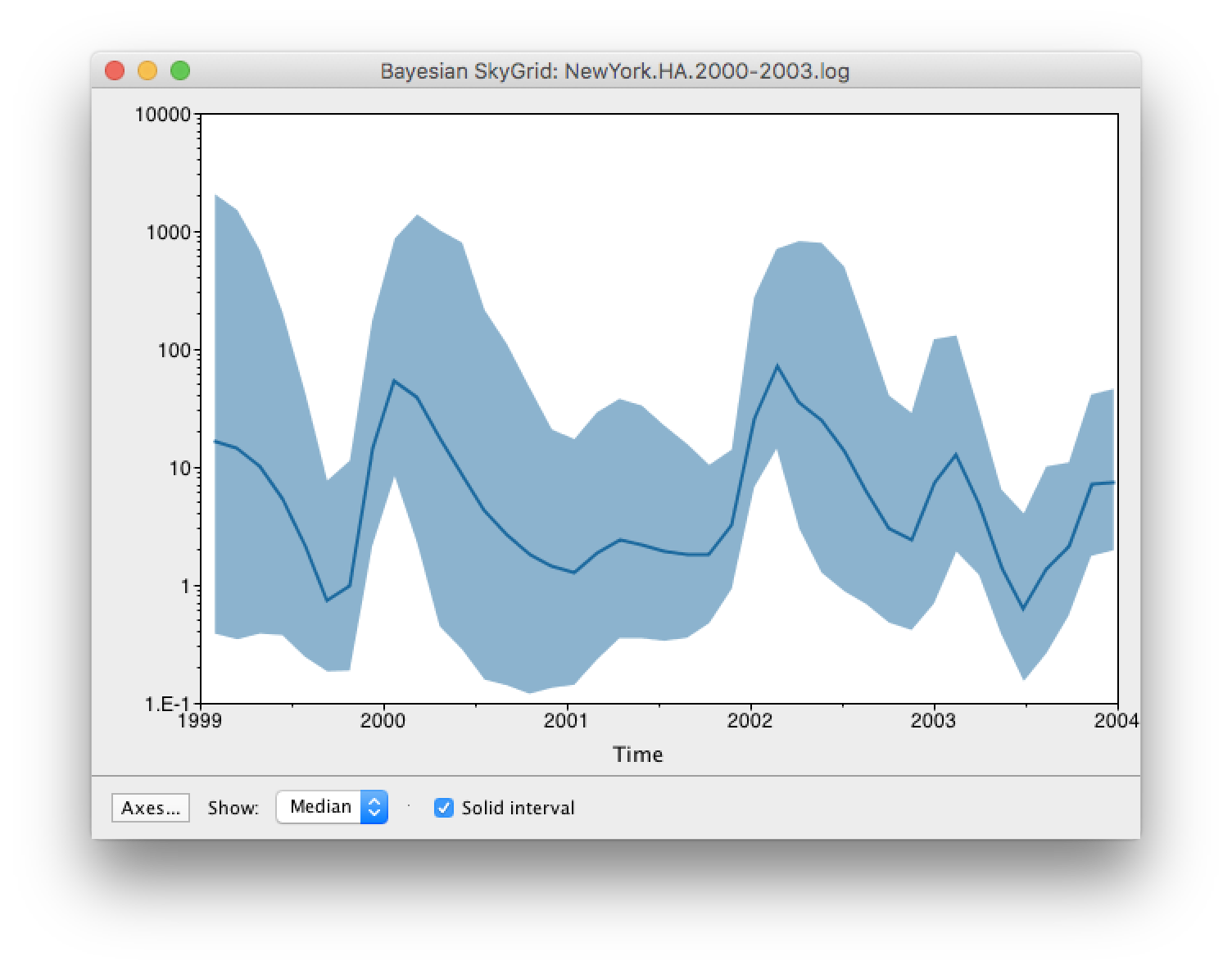
By default the y-axis is in a log scale. Press the Axes button and turn off Log axis for the Y axis. You will also need to set the Manual range because the upper HPD bounds will be very large. Set this to 0 to 100 and you get the following:
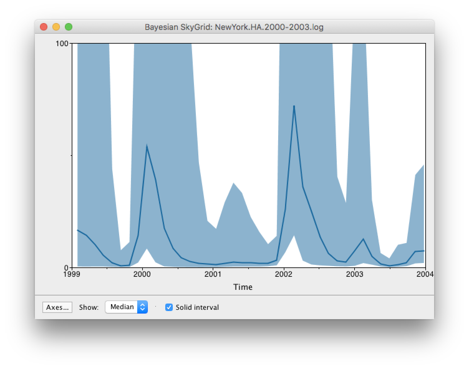
Here you can see that the seasonal peaks very strong (but that the uncertainty denoted by the credible intervale is also very large).
References
- Gill MS, Lemey P, Faria NR, Rambaut A, Shapiro B, and Suchard MA (2013) Improving Bayesian population dynamics inference: a coalescent-based model for multiple loci. Mol Biol Evol 30, 713-724.
- Minin VN, Bloomquist EW and Suchard MA (2008) Smooth Skyride through a Rough Skyline: Bayesian Coalescent-Based Inference of Population Dynamics. Molecular Biology and Evolution 25:1459-1471; doi:10.1093/molbev/msn090.
- Rambaut A, Pybus OG, Nelson MI, Viboud C, Taubenberger JK, Holmes EC (2008) The genomic and epidemiological dynamics of human influenza A virus. Nature, 453: 615-9.
Help and documentation
The BEAST website: http://beast.community
Tutorials: http://beast.community/tutorials
Frequently asked questions: http://beast.community/faq