In this tutorial, we will explore the use of the interactive graphical program TempEst (formerly known as Path-O-Gen) to examine virus sequence data that has been sampled through time to look for problematic sequences and to explore the degree and pattern of temporal signal. This can be a useful way of examining the data for potential issues before committing significant time to running BEAST.
Building a non-molecular clock tree
To examine the relationship between genetic divergence and time (temporal signal), we require a phylogenetic tree constructed without assuming a molecular clock. There is a wide range of suitable software packages (i.e., PhyML, RAxML, GARLI) but for this tutorial we are going to use IQ-Tree which uses a fast and effective stochastic algorithm to infer phylogenetic trees by maximum likelihood.
Install IQ-Tree using the instructions on the website and open a command-line prompt, navigating to the directory containing the data file ice_viruses.fasta.
To build a maximum likelihood phylogenetic tree using the GTR+gamma model type:
iqtree -s ice_viruses.fasta -m GTR+G
This will create a set of files in the directory containing various outputs and results:
ice_viruses.fasta.bionj
ice_viruses.fasta.ckp.gz
ice_viruses.fasta.iqtree
ice_viruses.fasta.log
ice_viruses.fasta.mldist
ice_viruses.fasta.treefile
ice_viruses.fasta.uniqueseq.phy
For our purposes we only need the maximum likelihood tree file ice_viruses.fasta.treefile. You can delete the other files if you like.
Running TempEst and loading the tree
Once running, TempEst will look similar irrespective of which computer system it is running on. For this tutorial, the Mac OS X version will be shown but the Linux & Windows versions will have exactly the same layout and functionality.
When started, TempEst will immediately display a file selection dialog box in which you can select the tree that you made in the previous section.
Select ice_viruses.fasta.treefile and click Open.
Parsing dates of sampling
Once the tree is loaded the main window will appear and look like this:
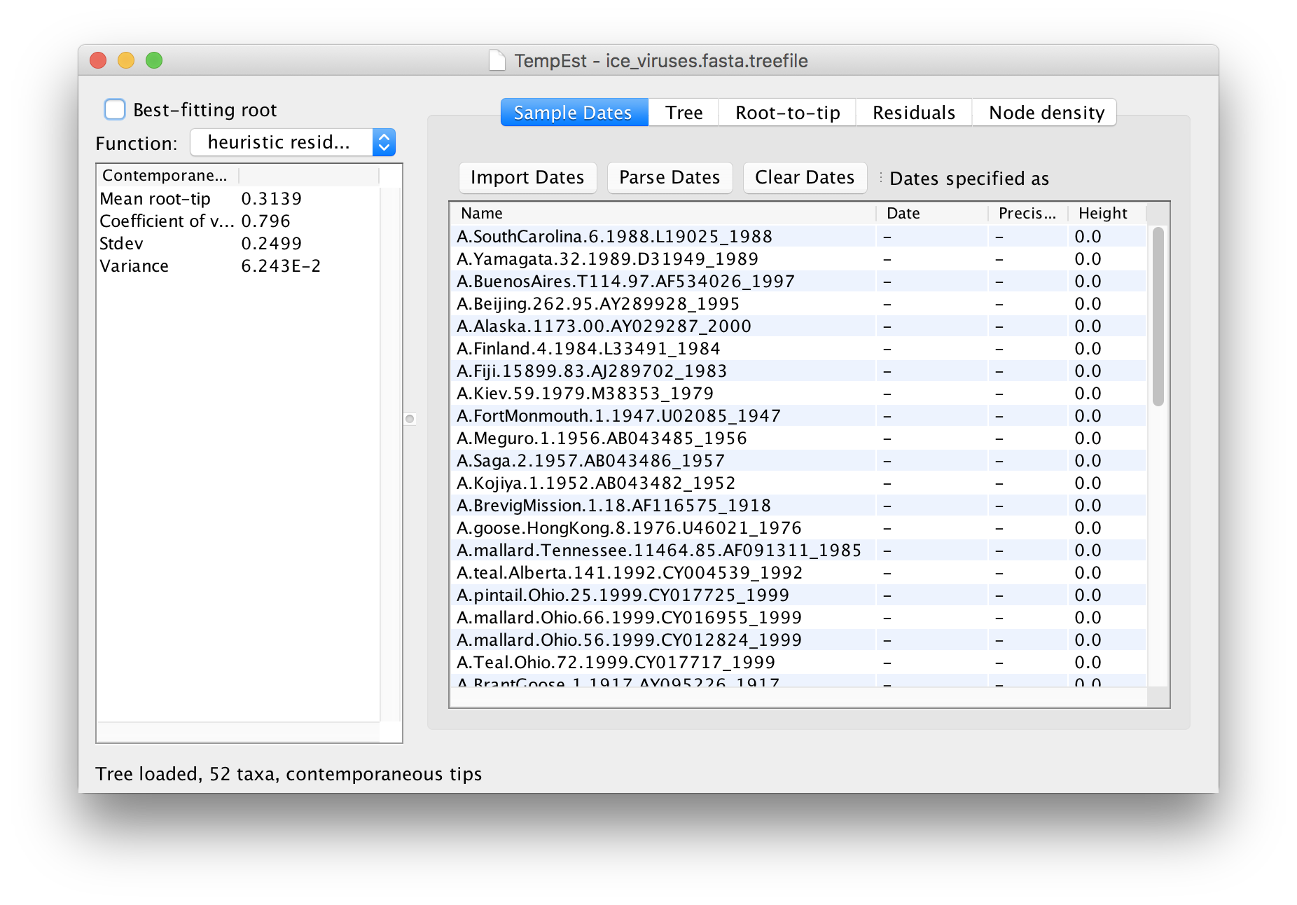
Ignore the panel on the left for the moment. The first thing that needs doing is to give the date of sampling to each of the sequences.
The actual year of sampling is given at the end of the name of each taxon. To specify the dates of the sequences in BEAUti we will use the Parse Dates button at the top of the panel. Clicking this will make a dialog box appear:

This operation attempts to extract the dates from the taxon names. It works by trying to find a numerical field within each name. This dialog box is the same as that in BEAUti and there are a wide range of options for doing this - See this page for details about the various options for setting dates in this panel. For these sequences you can set the options to look like the figure above: Defined just by its order, Order: last and Parse as a number option.
When parsing a number, you can ask BEAUti to add a fixed value to each date which can be useful for transforming a 2 digit year into a 4 digit year. Because all dates are specified in a four digit format in this case, no additional settings are needed. So, we can press OK.
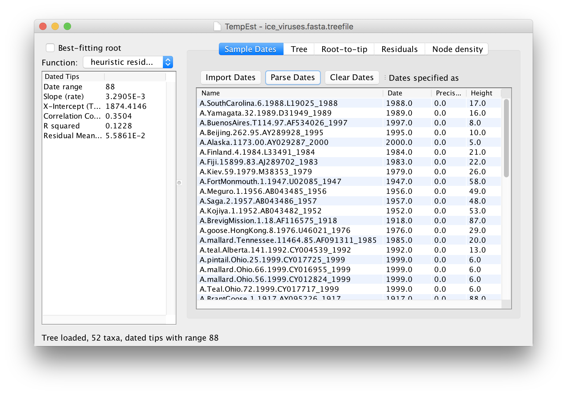
The table will now have the year of sampling for each virus in the Dates column. Click on the Dates column header to sort the dates and check that they are all correct.
The temporal signal and rooting
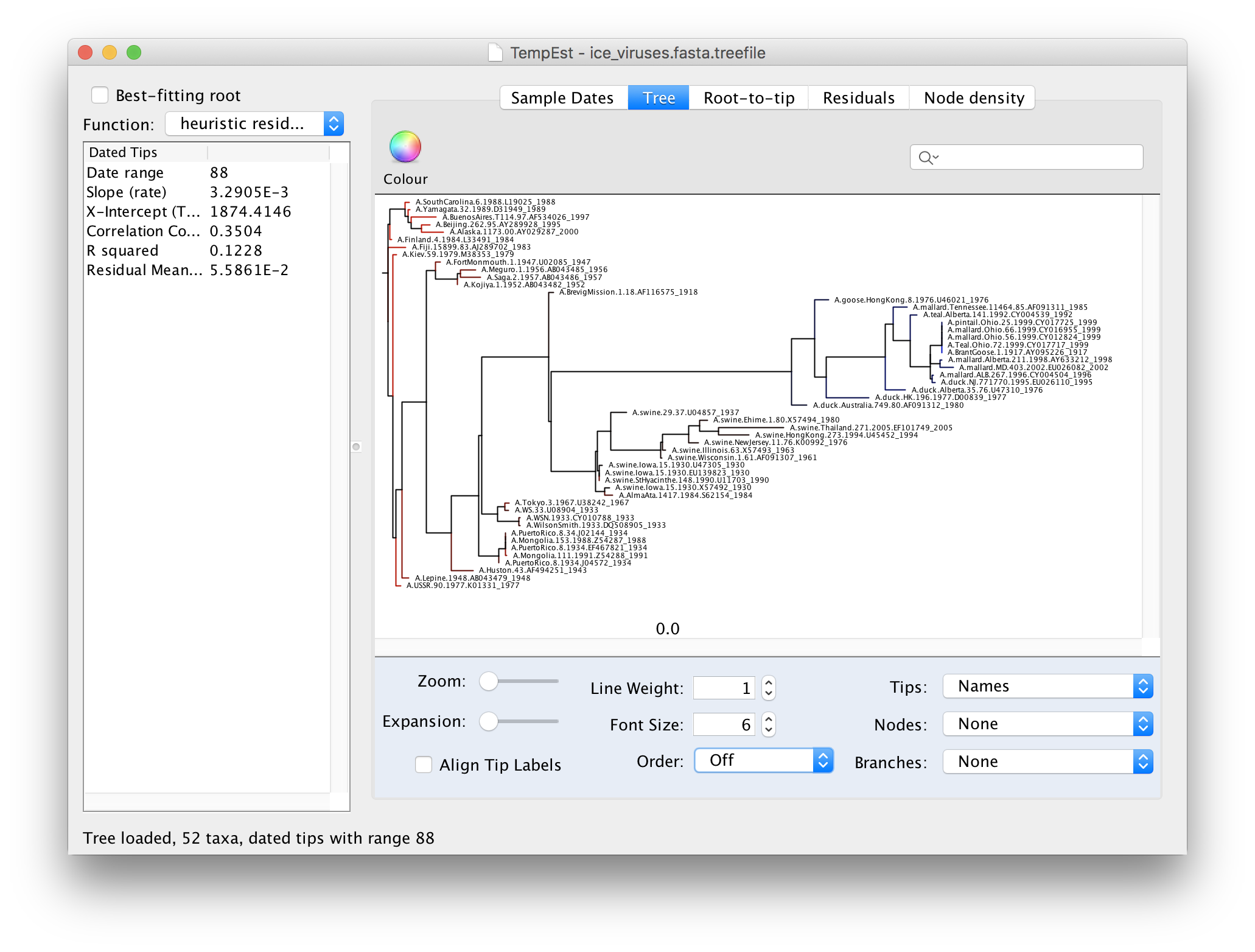
We can now explore the data using the tabs at the top of the window - Tree, Root-to-tip & Residuals. If you click on the Tree tab you will see the tree as loaded from the tree file. Because we constructed this tree using a non-molecular-clock model, it will be arbitrarily rooted. If you look at the date of each virus in the tree you will see that there is no correlation with the horizontal position:
Now switch to the Root-to-tip panel. This shows a plot of the divergence from the root of the tree against time of sampling (a so-called ‘Root to tip plot’):

You can see that there is very little correlation in this plot (the line is the best-fit regression). In the table on the left you can see the Correlation Coefficient is 0.35. This lack of correlation is expected as the root is arbitrarily set by the phylogeny reconstruction software and thus divergence from root is meaningless. TempEst can try to find the root of the tree that optimizes the temporal signal. It does this by trying all possible roots and picks the one that produces the optimal value of a range of statistics. The function it uses is selected in the menu at the top left.
The options are to minimize the mean of the squares of the residuals (residual-mean-squared), or to maximize the correlation coefficient (correlation) or R2 (R squared). These are all ad hoc procedures and no particular one is best but residual-mean-squared may be most consistent with the investigations here.
Click Best-fitting root to root the tree at the place that minimizes the mean of the squares of the residuals.

Now there is a better correlation between the dates of the tips and the divergence from the root (the correlation coefficient has nearly doubled). Return to the tree to look where the root was placed:
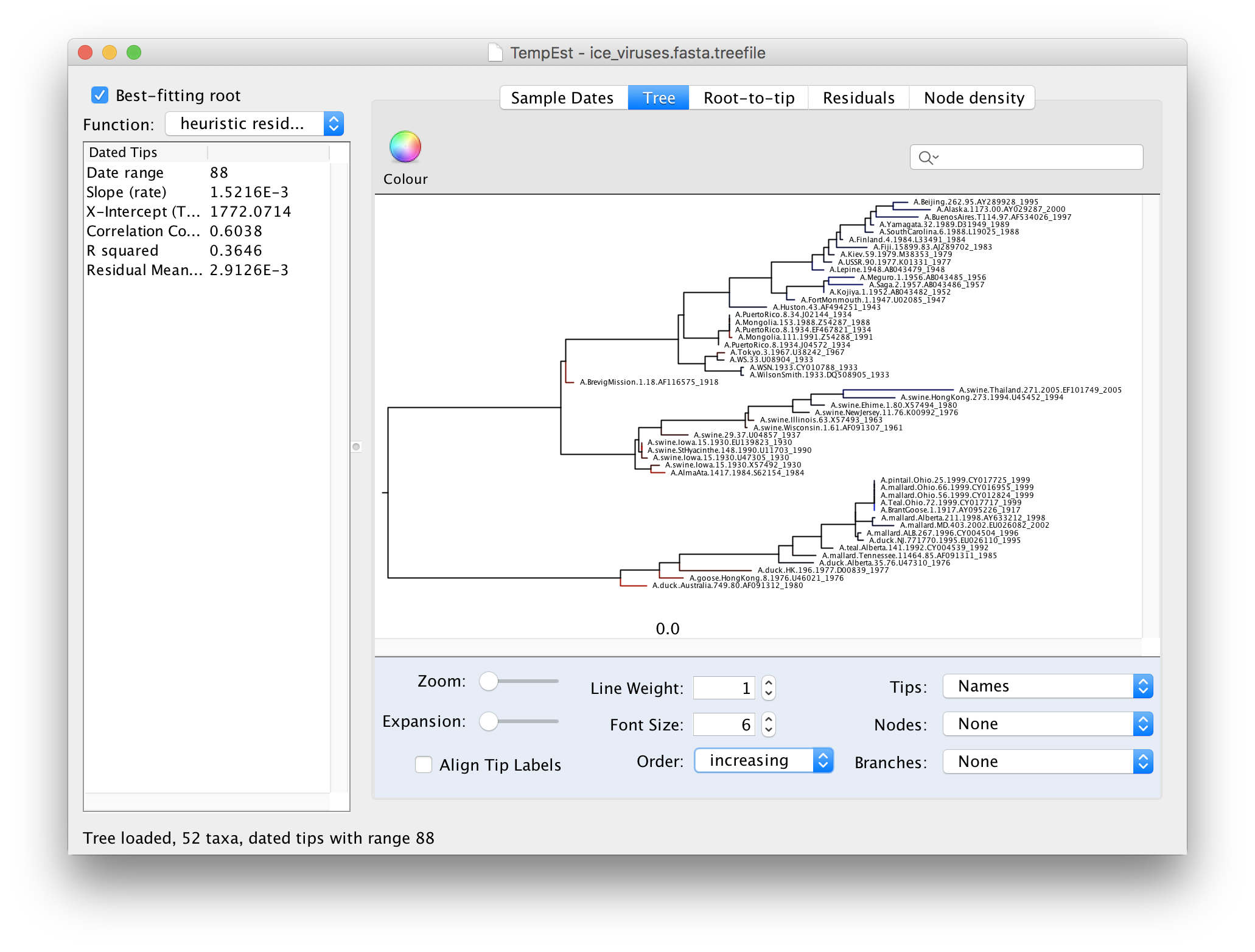
To make the tree easier to view, switch the Order option in the panel at the bottom to increasing. This rotates each node so the branch with the most tips is at the top. You can see now that there are 3 main lineages in this influenza tree - the human lineage at the top starting with the BrevigMission virus from 1918, the swine lineage in the middle and the avian lineage at the bottom.
The tree branches are coloured to show the residual with blue for tips with positive residuals (above the regression line), red for negative.
On the left hand side of the window there is a table of statistics:
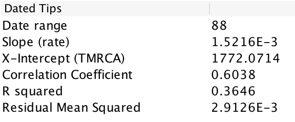
As well as the statistical metrics (Correlation Coefficient, R squared and Residual Mean Squared) there are the following:
Date range- The span of dates for the viruses.
Slope (rate)- The slope of the regression line. This is an estimate of the rate of evolution in substitutions per site per year.
X-Intercept (TMRCA)- The point on the x-axis at which the regression line crosses. This is an estimate of the date of the root of the tree.
Finding and interpreting problematic sequences
Switch to the Root-to-tip panel. Look for the point furthest from the line in the top left hand quadrant. If you click and drag your pointer over the point it will be highlighted in a blue colour:

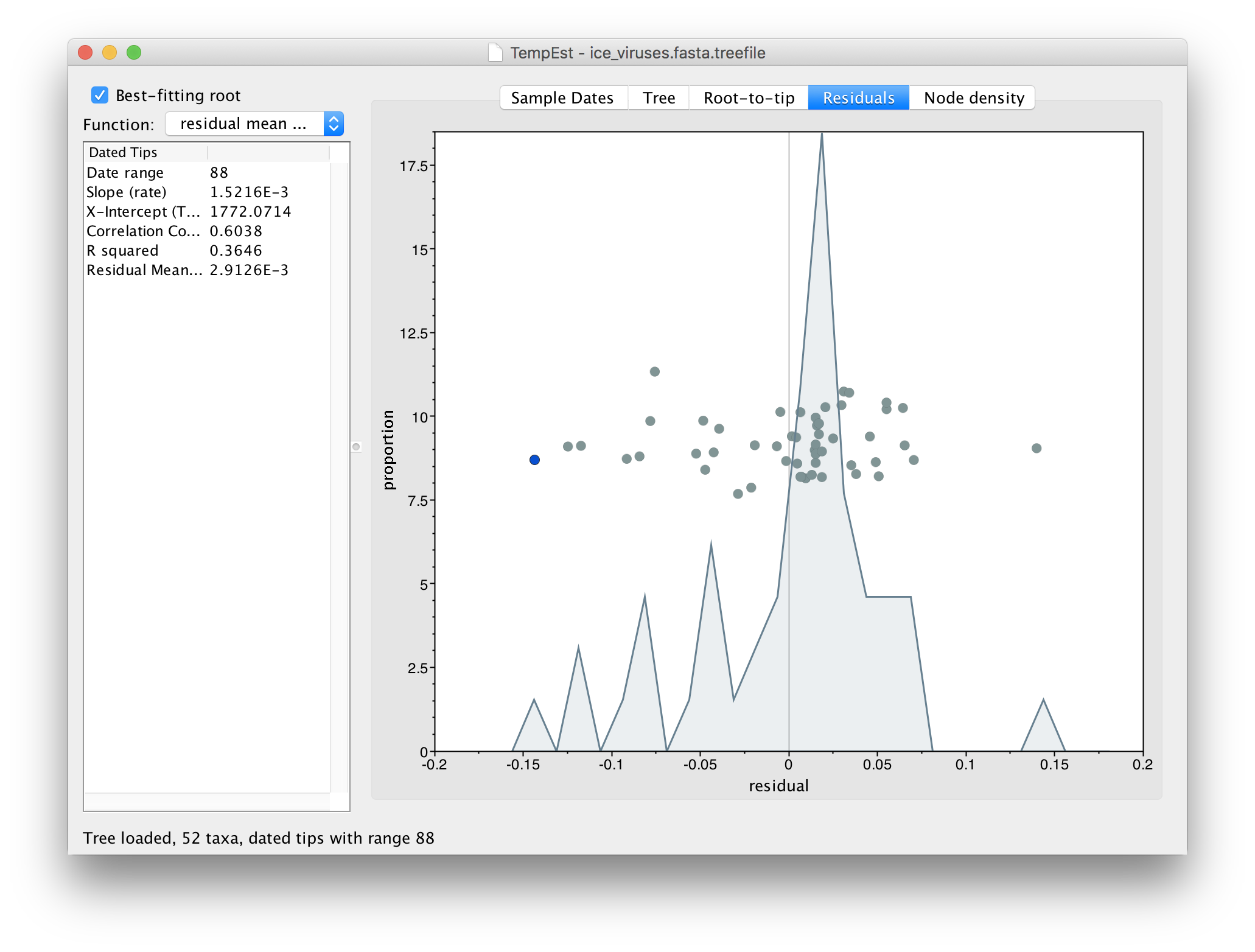
If you now switch to the Residual panel you will see a plot of all the residuals (the tangental deviation from the regression line). The virus we selected will still be highlighted and you can see it is an outlier. It is often easiest to select outliers in this plot.

If we now go back to the Tree panel you will see the label of the selected virus hilighted. You can use the Zoom slider in the bottom panel to zoom in on the area of the tree and the Font Size selector to increase the size of the label:
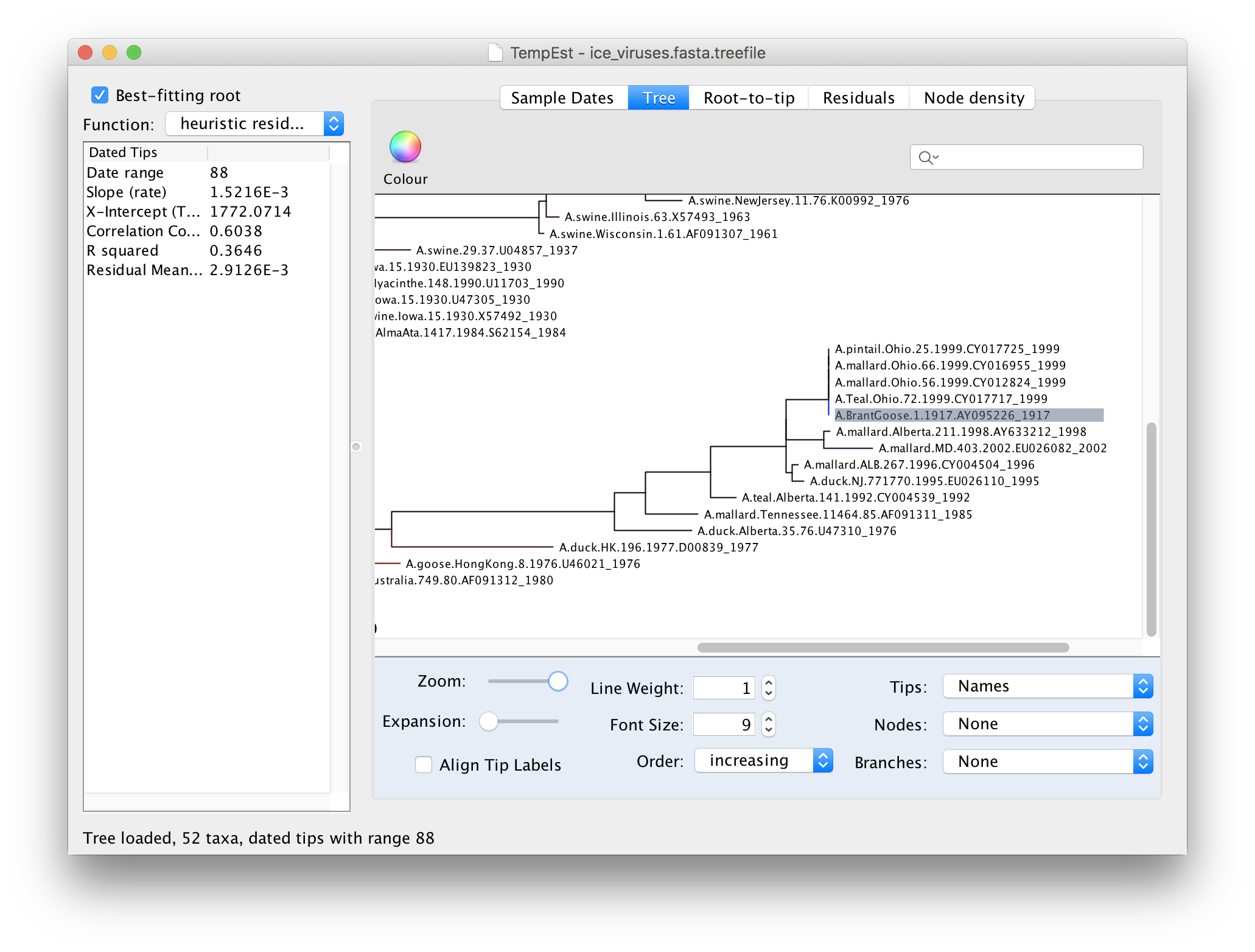
Looking at this part of the tree you should be able to see why A.BrantGoose.1.1917 is such an outlier. Although it is supposedly sampled from 1917, it is actually identical to a bunch of 4 other bird viruses from Ohio in 1999. This suggests that this virus sequence was the result of contamination by one of the other viruses in the same lab (another possibility is the mis-labelling of samples).
A.BrantGoose.1.1917, was published in a paper entitled ‘1917 Avian Influenza Virus Sequences Suggest that the 1918 Pandemic Virus Did Not Acquire Its Hemagglutinin Directly from Birds’. This paper used the fact that this sequence, from prior to the 1918 human pandemic, phylogenetically grouped with viruses from ‘modern’ birds to suggest that the 1918 pandemic was not a direct cross-over from birds. Clearly this interpretation is unsupported because of the likelihood of lab contamination as a source of the virus.One further tool is available that can be useful to find problematic sequences. Turn on the Show ancestor traces option at the bottom of the panel:
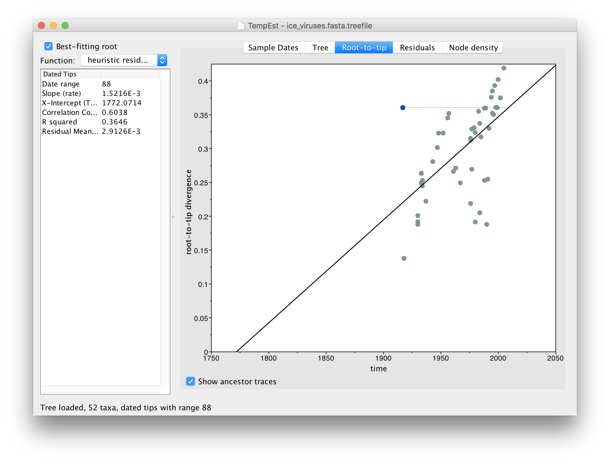
This option draws a green line from the selected virus to the point on the regression line where the immediate ancestor should lie (i.e., given its divergence from the root). If the line, like the example here, is horizontal and extends to the left, this suggests the sequence is actually more recent than the date that it has been given. This may be indicative of contamination from a recent virus than the supposed date or a mislabelling (another issue is that the date format could be wrongly parsed).
Ancestor lines that are vertical upwards suggest that the sequence has too many unique differences compared to its ancestor. This may be indicative of sequencing error, degraded samples, host restriction-factor editing, alignment issues, or recombination.
Ancestor lines that are horizontal and to the right mean that the supposed date of the virus is more recent than the divergence would suggest. This can be due to contamination by an older virus (or a mislabelling).
The ancestor lines can never be downwards as this would denote a negative divergence. Shorter ancestor lines and ones that lie close to the regression gradient are less likely to be problematic.
Go to the Residuals panel and select the most left hand (negative) residual point:
Then return to the tree and examine the selected virus:
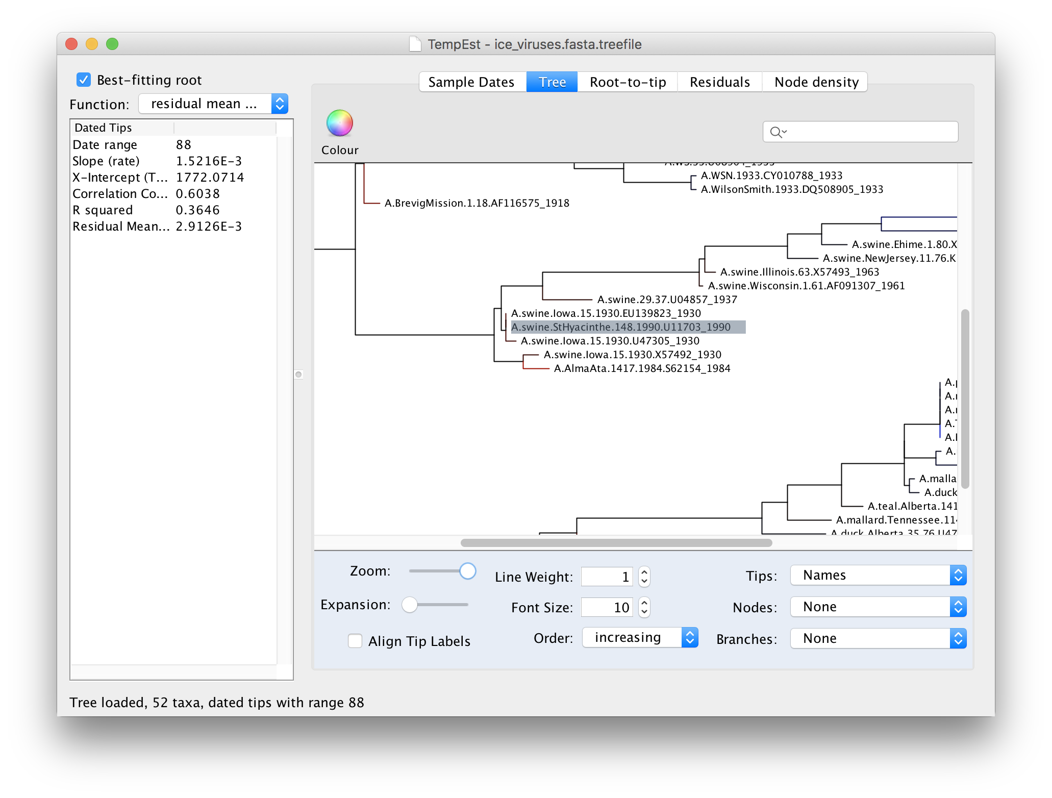
You can see here that the selected virus, A.swine.StHyacinthe.148.1990, although supposedly from 1990, is identical to a virus from Iowa in 1930. A/swine/Iowa/15/1930 is a commonly used lab virus and thus this is likely, again, a contamination issue.
A.swine.StHyacinthe.148.1990 is correct, it would mean that this virus is directly descended from the 1930s viruses but hasn’t evolved at all in this time. This would require the virus to have been frozen and then re-emerge 60 years later. Although this is not entirely implausible it is unlikely to have happened in this case.There are 4 other examples of this type of problematic sequences in this data set. See if you can identify them.
Cleaning the data set
Once all of the problematic sequences have been identified, these can be removed from the alignment and the tree rebuilt to see the effect they were having onb the analysis. Download the file, ice_viruses_cleaned.fasta, which has had 7 problematic sequences removed.
Using the instructions given above, for the file ice_viruses_cleaned.fasta, repeat the tree building procedure using IQ-Tree, load the resulting tree into TempEst and parse the dates for each virus. Switch to the Root-to-tip panel, turn on Best-fitting root and compare the plot to the one you got before. You should see something like this:

You can see that the correlation between divergence from root and time of sampling is much better (the Correlation Coefficent in the table on the left is now 0.733).
You will notice that the relationship is still not very clean. The reason for this is that there are 3 different lineages here (human, swine and avian) and that combining them all into a single tree (which is then fixed) may obscure their individual patterns.
The final file in this analysis, ice_viruses_human.fasta, is one that contains only the human viruses.
Repeating the steps above to build a tree and load it into TempEst now shows this relationship:
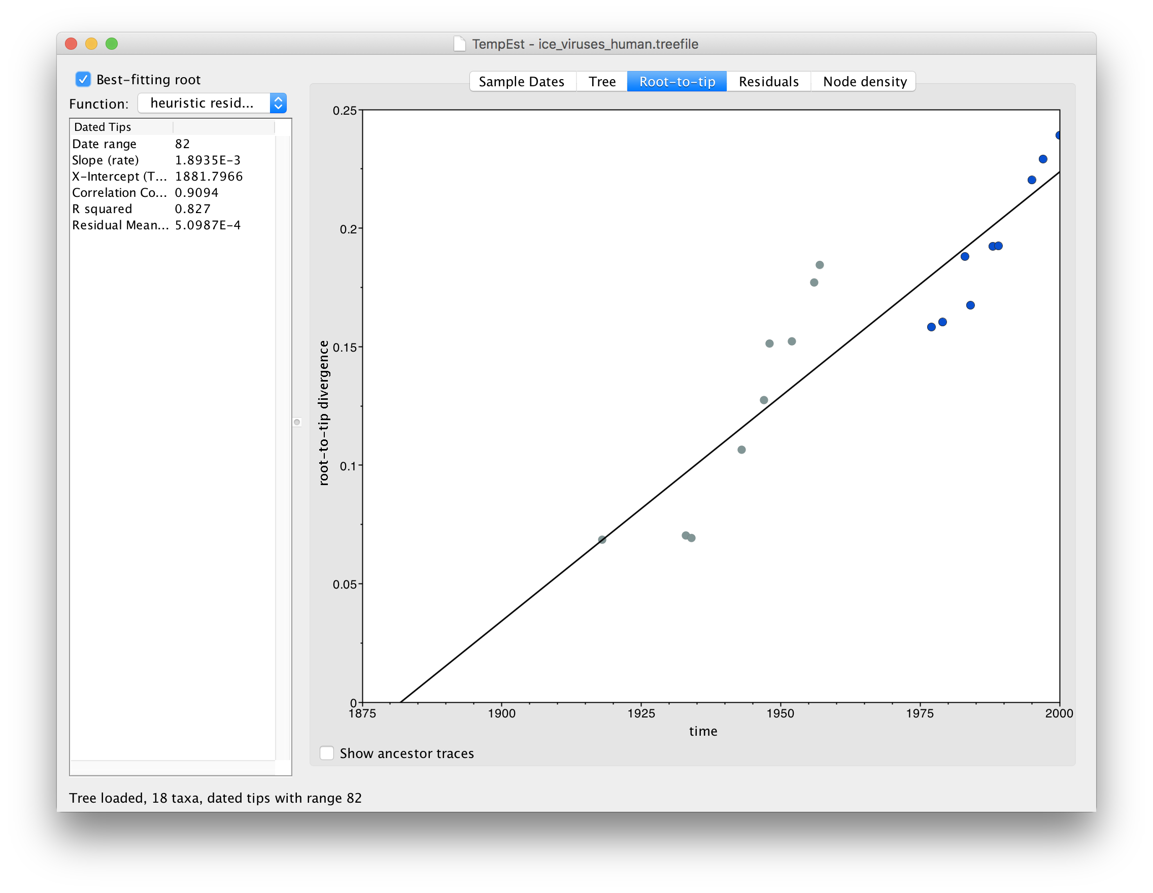
In this image everything after 1975 is highlighted in blue. What you should be able to see is that there are actually two lines of points here, one from 1918 to 1957 and one from 1977 to 2000. There is a gap in time (in the horizontal axis) of about 20 years but no gap in the divergence from the root.