Introduction
The first step will be to convert a NEXUS file with a DATA or CHARACTERS block into a BEAST XML input file. This is done using the program BEAUti (this stands for Bayesian Evolutionary Analysis Utility). This is a user-friendly program for setting the evolutionary model and options for the MCMC analysis. The second step is to actually run BEAST using the input file that contains the data, model and settings. The final step is to explore the output of BEAST in order to diagnose problems and to summarize the results.
To undertake this tutorial, you will need to download three software packages in a format that is compatible with your computer system (all three are available for Mac OS X, Windows and Linux/UNIX operating systems):
The data are 71 sequences from the prM/E gene of yellow fever virus (YFV) from Africa and the Americas with isolation dates ranging from 1940-2009. The sequences represent a subset of the data set analyzed by Bryant et al. (Bryant JE, Holmes EC, Barrett ADT, 2007 Out of Africa: A Molecular Perspective on the Introduction of Yellow Fever Virus into the Americas. PLoS Pathog 3(5): e75).
Loading the data into BEAUti
To load a NEXUS format alignment, simply select the Import Data... option from the File menu and select the file called YFV.nex.
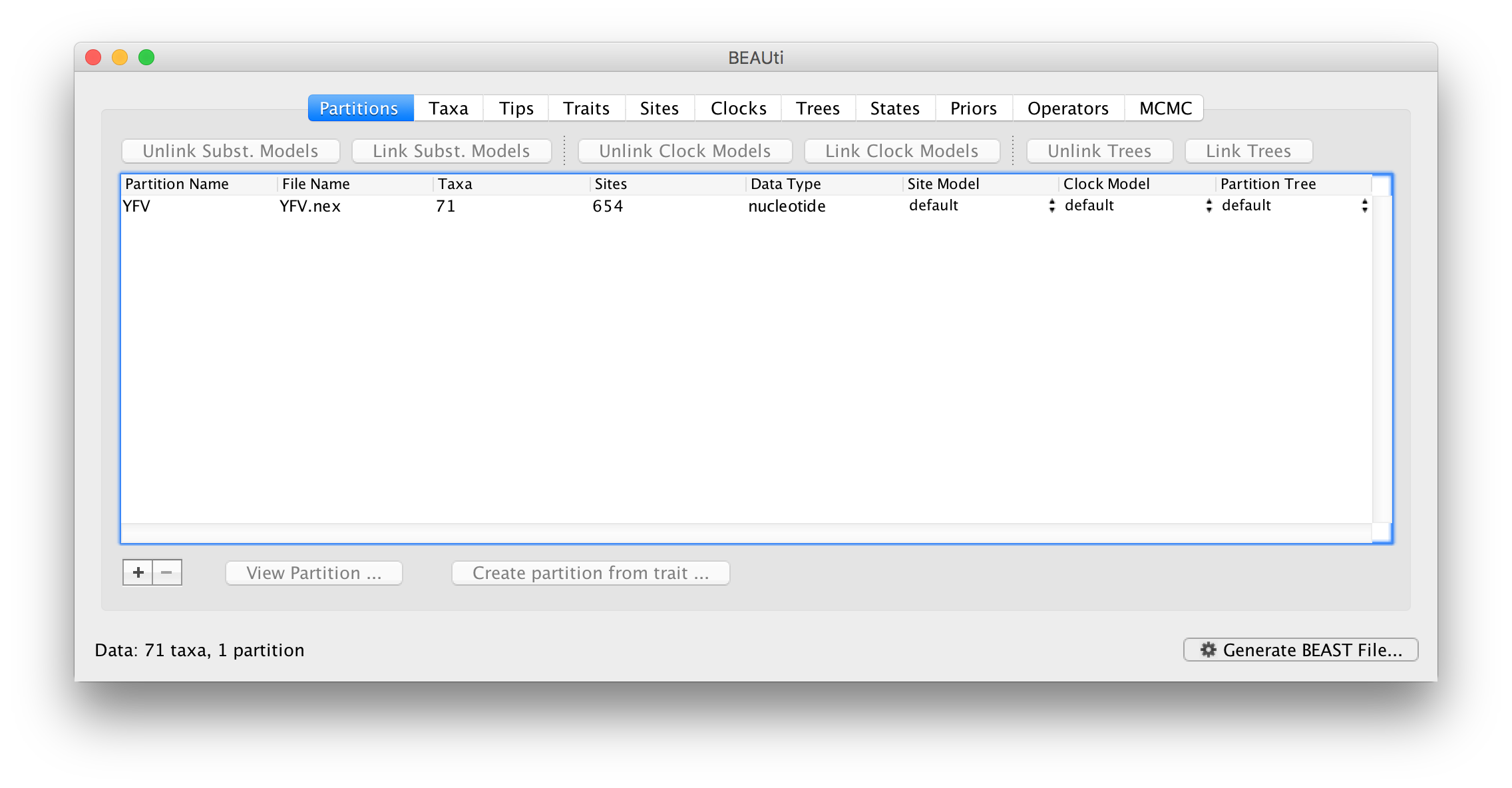
This file contains an alignment of 71 sequences from the prM/E gene of YFV, 654 nucleotides in length.
Once loaded, the sequence data will be listed under Data Partitions:
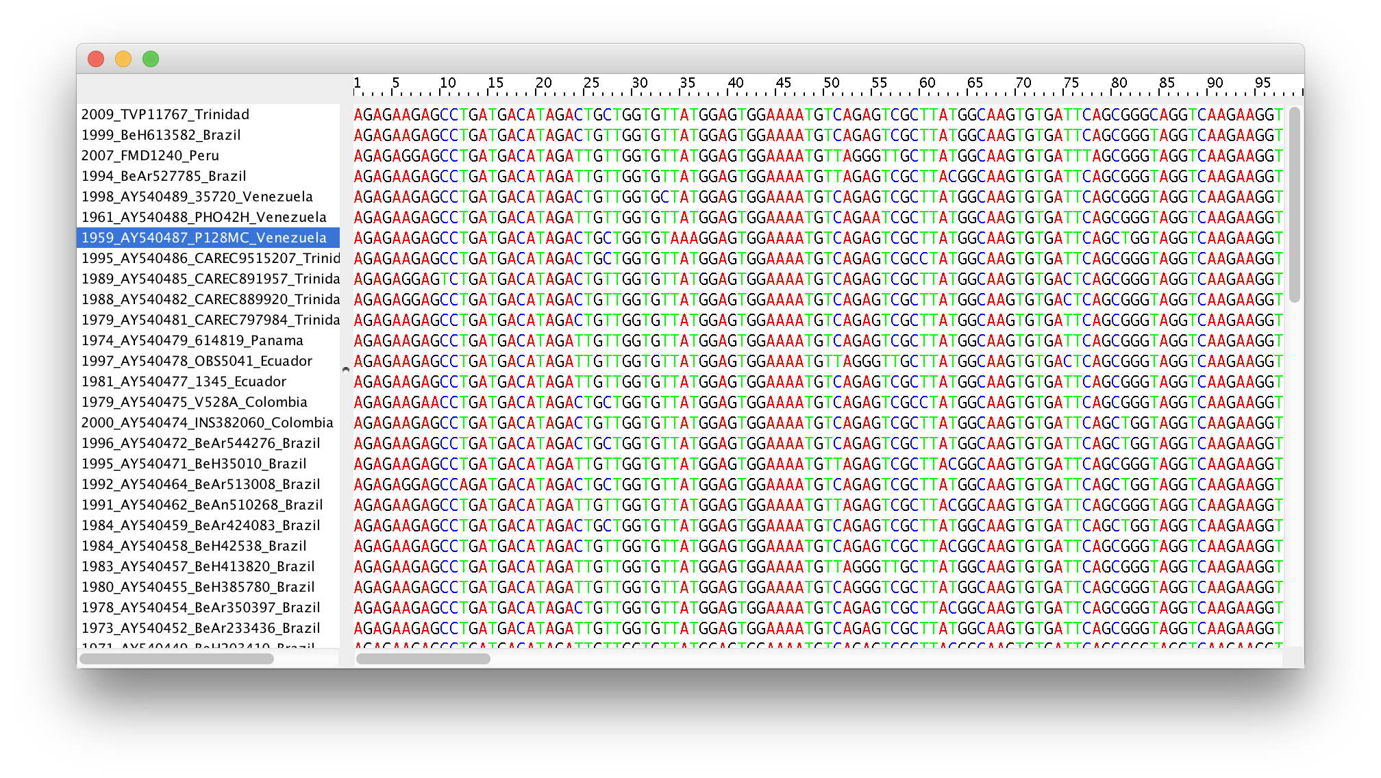
Double-click on the File Name in the table (but not on Partition Name) to display the actual sequence alignment:
Specifying a taxon set
Under the Taxa panel, we can define sets of taxa for which we would like to obtain particular statistics, enforce a monophyletic constraint, or put calibration information on.
Let’s define an “Americas” taxon set by pressing the small “plus” button at the bottom left of the panel:
This will create a new taxon set.
Rename it by double-clicking on the entry that appears (it will initially be called untitled1).
Call it Americas.
Do not enforce monophyly using the monophyletic? option because we will evaluate the support for this cluster.
We do not opt for the includeStem? option either because we would like to estimate the TRMCA for the viruses from the Americas and not for the parent node leading to this clade.
In the next table along you will see the available taxa.
Taxa can be selected and moved to the Included taxa set by pressing the green arrow button.
Note that multiple taxa can be selected simultaneously holding down the Command or Control button on a Mac or PC, respectively.
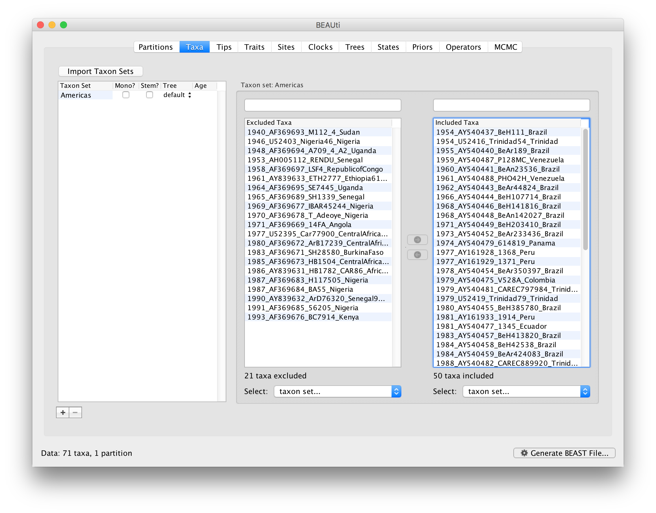
Since most taxa are from the Americas, the most convenient is to simply select all taxa, move them to the Included taxa set, and then move back the African taxa (the country of sampling is included at the end of the taxa names). Check there are only African countries on the left (there should be 21) and only American countries on the right (there should be 50).
For more information on creating taxon sets, see this page.
After these operations, the screen should look like this:
Setting the tip dates
To inform BEAUti/BEAST about the sampling dates of the sequences, go to the Tips panel and select the Use tip dates option. By default all the taxa are assumed to have a date of zero (i.e. the sequences are assumed to be sampled at the same time; BEAST considers the present or most recent sampling time as time 0). In this case, the YFV sequences have been sampled at various dates going back to the 1940s. The actual year of sampling is given in the name of each taxon and we could simply edit the value in the Date column of the table to reflect these. However, if the taxa names contain the calibration information, then a convenient way to specify the dates of the sequences in BEAUti is to use the Parse Dates button at the top of the Tips panel. Clicking this will make a dialog box appear:
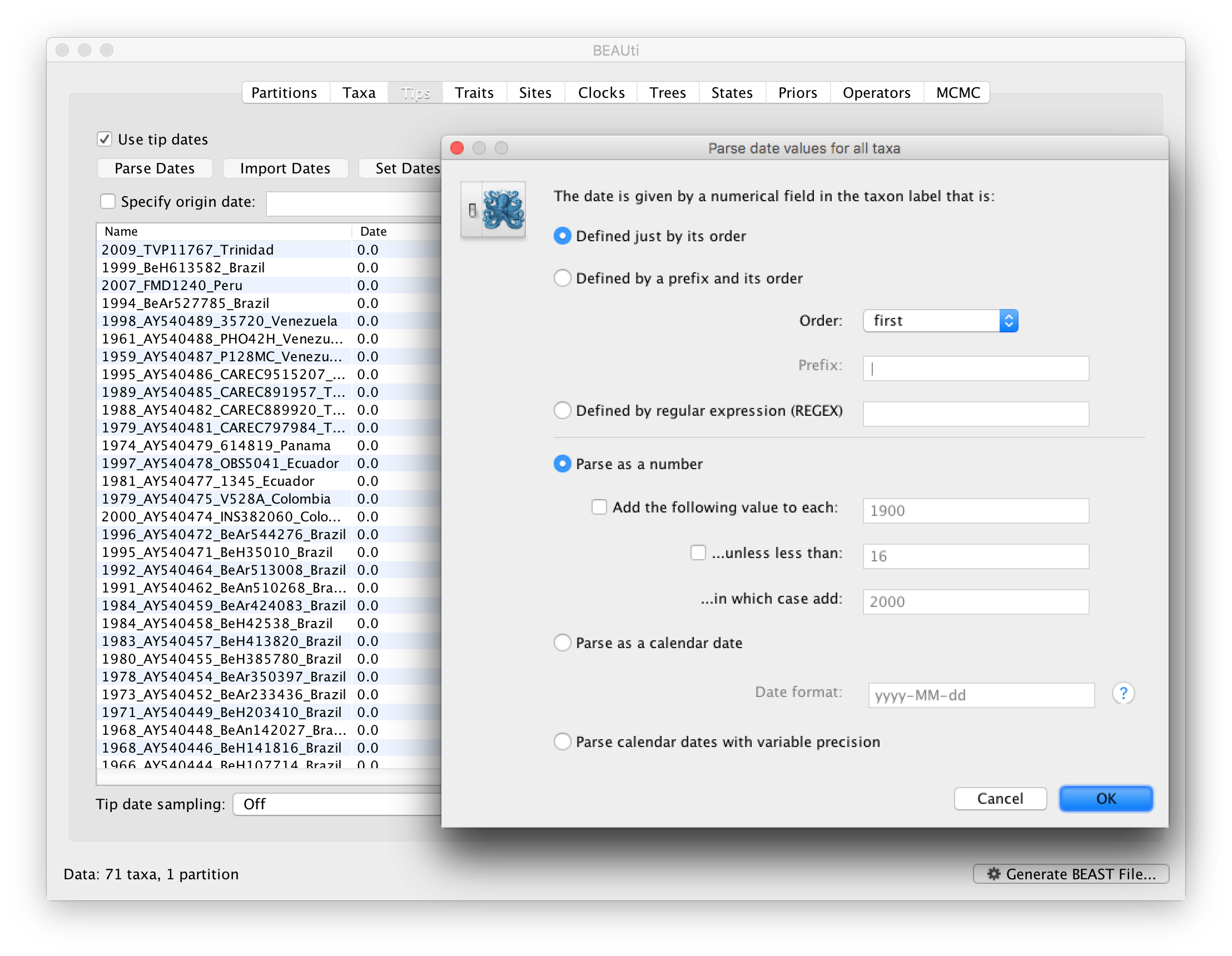
This operation attempts to guess what the dates are from information contained within the taxon names. It works by trying to find a numerical field within each name. If the taxon names contain more than one numerical field (such as the some YFV sequences, above) then you can specify how to find the one that corresponds to the date of sampling. See this page for details about the various options for setting dates in this panel. For the YFV sequences you can keep the default Defined just by its order and Order: first (but make sure that the Parse as a number option is selected).
When parsing a number, you can ask BEAUti to add a fixed value to each date which can be useful for transforming a 2 digit year into a 4 digit year. Because all dates are specified in a four digit format in this case, no additional settings are needed. So, we can press OK.
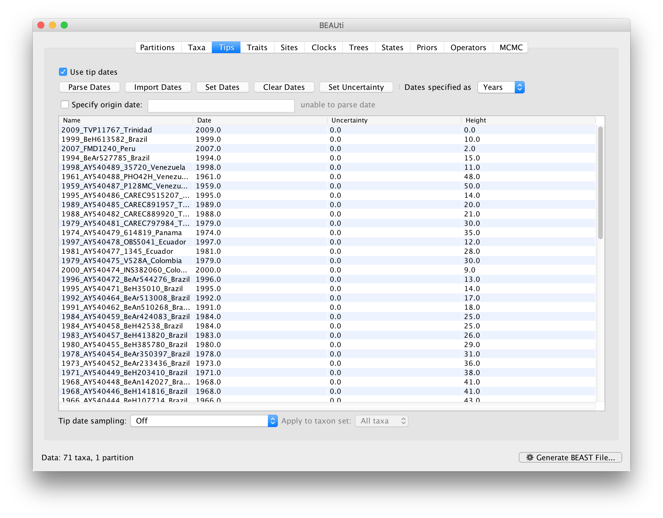
The Height column lists the ages of the tips relative to time 0 (in our case 2009).
For these sequences, only the sampling year is provided and not the exact sampling dates. This uncertainty will negligible with respect to the relatively large evolutionary time scale of this example, however, it is possible to accommodate the sampling time uncertainty — see here.
Setting the evolutionary model
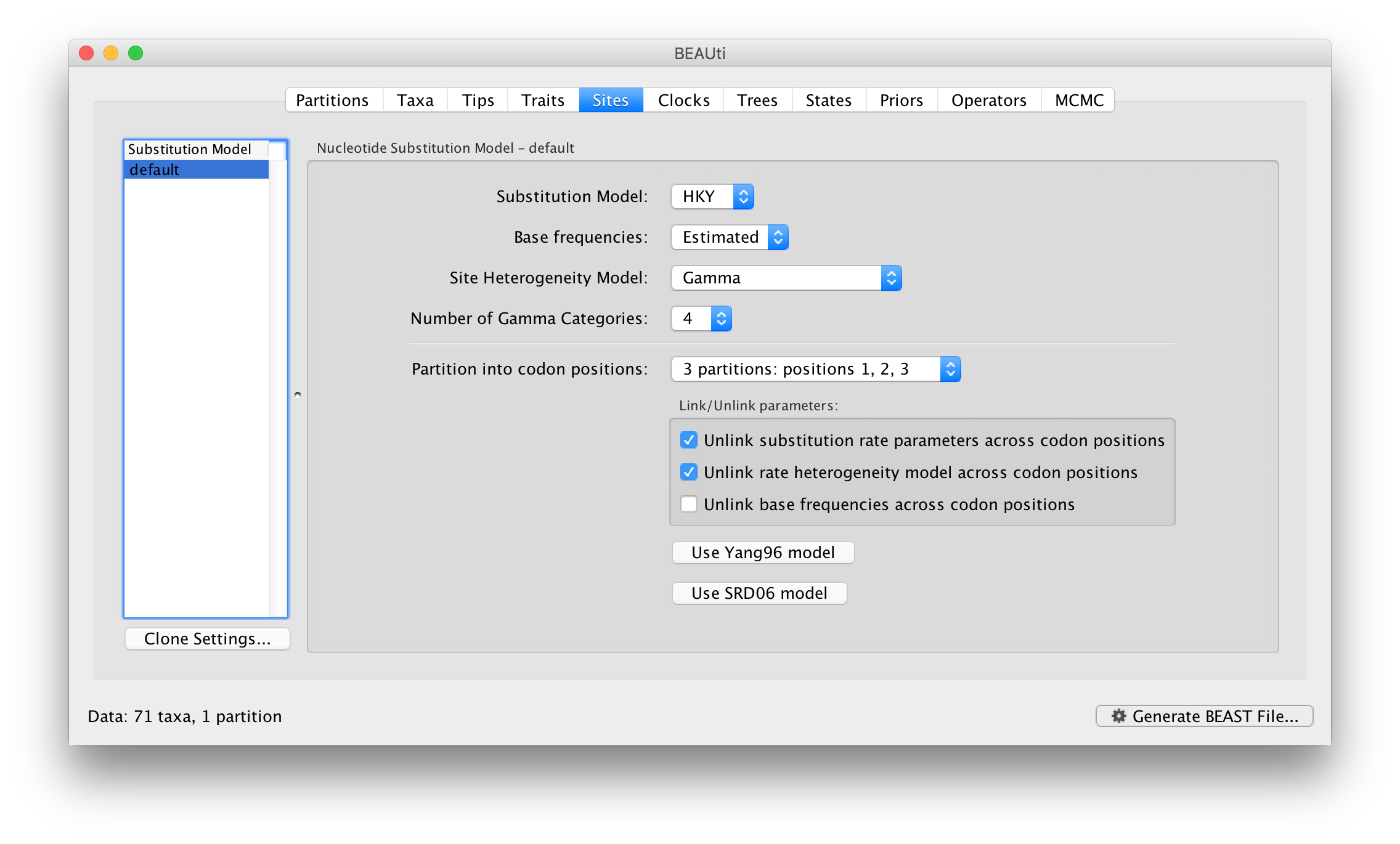
The next thing to do is to click on the Sites tab at the top of the main window. This will reveal the evolutionary model settings for BEAST. Exactly which options appear depend on whether the data are nucleotides or amino acids (or traits). This tutorial assumes that you are familiar with the evolutionary models available — however there are a couple of points to note about selecting a model in BEAUti:
- Substitution Model:
- For nucleotide data, this is a choice of
JC,HKY,GTRorTN93. Other substitution models are possible by constraining one of these model. See this page for more details. - Base frequencies:
- The nucleotide base frequencies can be
Estimated(estimated as a parameter in the model),Empirical(estimated emprically from the data and then fixed) orAll equal(fixed to be 0.25 each). - Site Heterogeneity Model:
- A choice of the discrete gamma distribution model, the invariant site model or both.
- Partition into codon positions:
- Selecting the
Partition into codon positionsoption assumes that the data are aligned as codons. This option will then estimate a separate rate of substitution for each codon position, or for 1+2 versus 3, depending on the setting. - Unlink substitution model across codon positions:
- Selecting the
Unlink substitution model across codon positionswill specify that BEAST should estimate a separate transition-transversion ratio or general time reversible rate matrix for each codon position. - Unlink rate heterogeneity model across codon positions:
- Selecting the
Unlink rate heterogeneity model across codon positionswill specify that BEAST should estimate set of rate heterogeneity parameters (gamma shape parameter and/or proportion of invariant sites) for each codon position. - Unlink base frequencies across codon positions:
- Selecting the
Unlink base frequencies across codon positionswill specify that BEAST should estimate a separate set of base frequencies for each codon position.
For this tutorial, select the 3 partitions: positions 1, 2, 3 option so that each codon position has its own HKY substitution model, rate of evolution, Estimated base frequencies, and Gamma-distributed rate variation among sites (equal weights):
Setting the clock model
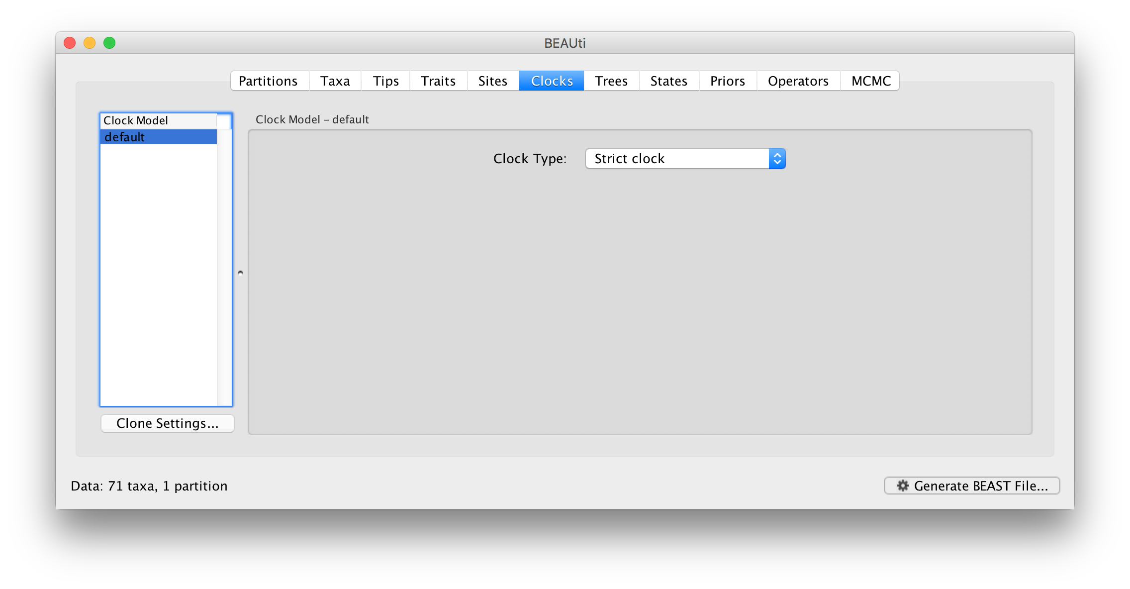
Click on the Clocks tab at the top of the main window. We will perform our initial run using the (default) strict molecular clock model:
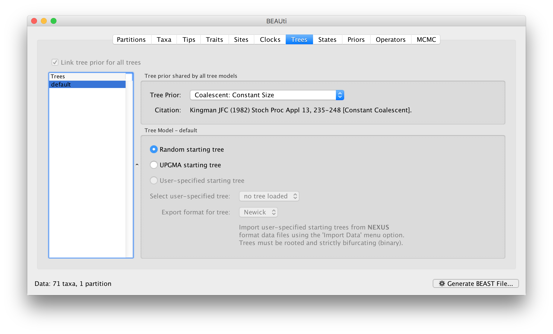
Setting the starting tree and tree prior
Click on the Trees tab at the top of the main window. We keep a default random starting tree and a (simple) constant size coalescent prior. The tree priors (coalescent and other models) are described on this page.
Setting up the priors
Review the prior settings under the Priors panel:
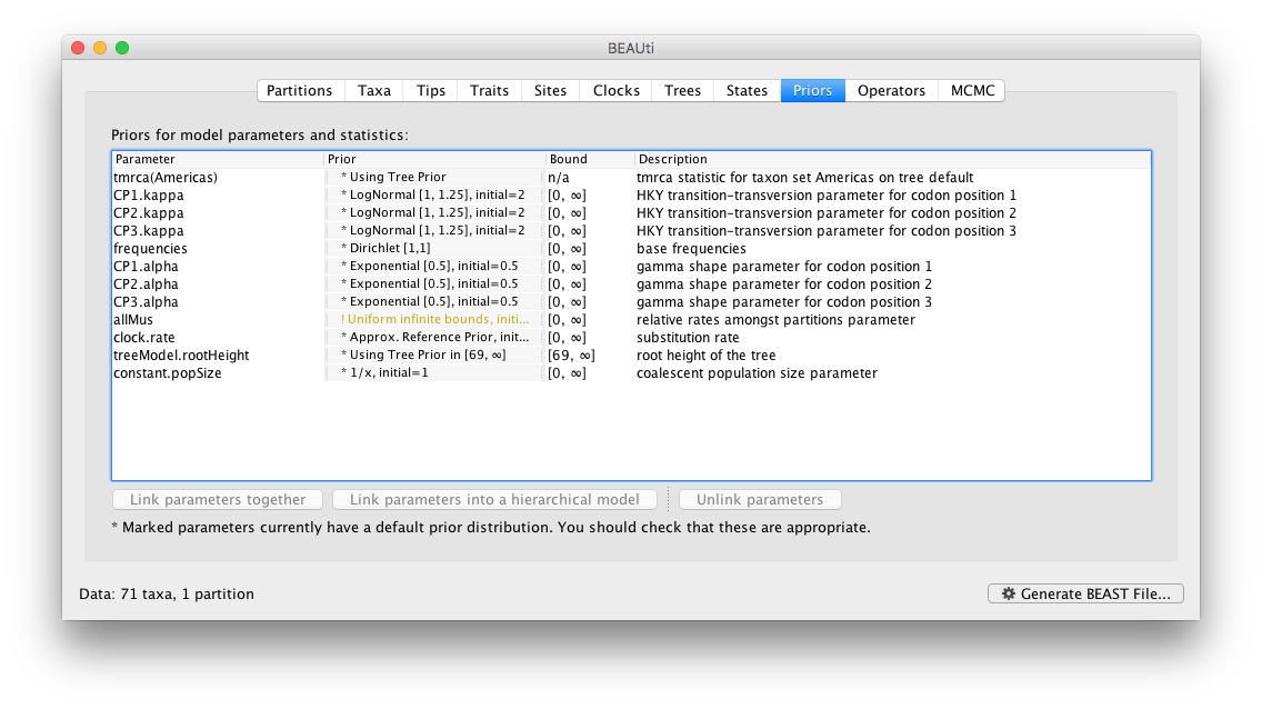
In this case, all priors on continuous parameters are proper priors (priors that integrate to 1).
Note that the default prior on the rate of evolution (clock.rate) is an approximation of a conditional reference prior (Approx. Reference Prior) (Ferreira and Suchard, 2008). If the sequences are not associated with different sampling dates (they are contemporaneous), or when the sampling time range is trivial for the evolutionary scale of the taxa, the substitution rate can be fixed to a value based on another source, or better, a prior distribution can be specified to also incorporate the uncertainty of this ‘external’ rate. Fixing the rate to 1.0 will result in the ages of the nodes of the tree being estimated in units of substitutions per site (i.e. the normal units of branch lengths in popular packages such as MrBayes). Note that when selecting to fix the rate to a value, the transition kernel(s) on this parameter (Operators panel, see next section) will be automatically unselected.
Setting up the operators
Each parameter in the model has one or more “operators” (these are variously called moves, proposals or transition kernels by other MCMC software packages such as MrBayes and LAMARC). The operators specify how the parameters change as the MCMC runs. For this analysis, no changes are required to this table.

Setting the MCMC options
The MCMC tab in BEAUti provides settings to control the MCMC chain. Firstly we have the Length of chain. This is the number of steps the MCMC will make in the chain before finishing. How long this should depend on the size of the dataset, the complexity of the model and the precision of the answer required. The default value of 10,000,000 is entirely arbitrary and should be adjusted according to the size of your dataset. We will see later how the resulting log file can be analyzed using Tracer in order to examine whether a particular chain length is adequate.
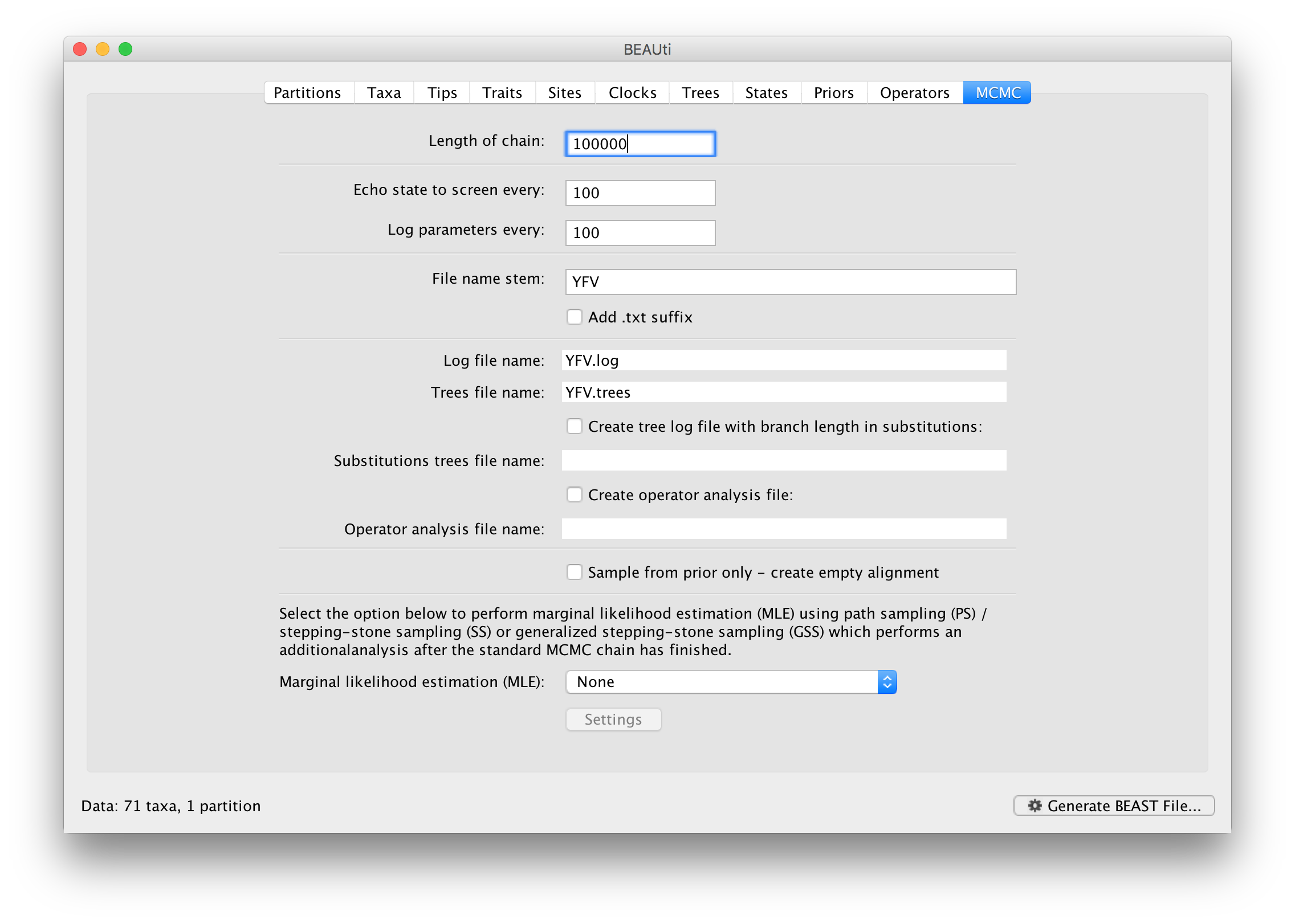
The next couple of options specify how often the current parameter values should be displayed on the screen and recorded in the log file. The screen output is simply for monitoring the program’s progress so can be set to any value (although if set too small, the sheer quantity of information being displayed on the screen will slow the program down). For the log file, the value should be set relative to the total length of the chain. Sampling too often will result in very large files with little extra benefit in terms of the precision of the estimates. Sample too infrequently and the log file will not contain much information about the distributions of the parameters. You probably want to aim to store no more than 10,000 samples so this should be set to something >= chain length / 10,000.
For this dataset let’s initially set the chain length to 100,000 as this will run reasonably quickly on most modern computers. Although the suggestion above would indicate a lower sampling frequency, in this case set both the sampling frequencies to 100.
Echo state to screen option to 10000 resulting in only 100 updates to the screen as the analysis runs.Below the parameter logging frequency, you can set the checkpointing frequency. Checkpointing is a mechanism that allows store the state of a computation in a way that allows it be continued at a later time without changing the computation’s behavior. This is useful when a run is interrupted for some reason or when you would simply like to continue a run that ended, but has not provided sufficient samples.
The next option allows the user to set the File stem name; if not set to ‘YFV’ by default, you can type this in here (or add more detail about the analysis). The next two options give the file names of the log files for the parameters and the trees. These will be set to a default based on the file stem name.
.txt to the log and the trees file — Windows will hide the .txt but still show you the .log and .trees extensions so you can distinguish the files.The remaining options can be left unselected this time. An option is available to sample from the prior only, which can be useful to evaluate how divergent our posterior estimates are when information is drawn from the data. Also, one can chose to perform marginal likelihood estimation to assess model fit; we will return to this in a later tutorial.
Saving and Loading BEAUti files
If you select the Save option from the File menu this will save a document in BEAUti’s own format. Note that is not in the format that BEAST understands — it can only be reopened by BEAUti. The idea is that the settings and data in BEAUti can be saved and loaded at a later time. We suggest you save BEAUti files with the extension ‘.beauti’.
Generating the BEAST XML file
We are now ready to create the BEAST XML file. Select Generate XML... from the File menu (or the button at the bottom of the window). BEAUti will ask you to review the prior settings one more time before saving the file (and will indicate if any are improper). Continue and choose a name for the file — it will offer the name you gave it in the MCMC panel and we usually end the filename with ‘.xml’ (although see the note, above, about extensions on Windows machines – you may want to give the file the extension ‘.xml.txt’).
Running BEAST
We are now ready to run the file through BEAST.
The following dialog box will appear:
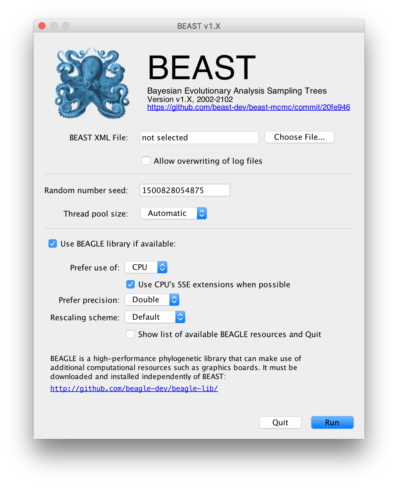
All you need to do is to click the Choose File... button, select the XML file you created in BEAUti, above, and press Run. For information about the other options see the page on the BEAST program.
When you press Run BEAST will load the XML file, setup the analysis and then run it with no further interaction. In the output window you will see lots of information appearing. It starts by printing the title and credits:
      BEAST X v10.5.0 Prerelease #94f74eb37, 2002-2024
       Bayesian Evolutionary Analysis Sampling Trees
                 Designed and developed by
   Alexei J. Drummond, Andrew Rambaut and Marc A. Suchard

               Department of Computer Science
                   University of Auckland
                  alexei@cs.auckland.ac.nz

             Institute of Ecology and Evolution
                  University of Edinburgh
                     a.rambaut@ed.ac.uk

              David Geffen School of Medicine
           University of California, Los Angeles
                     msuchard@ucla.edu

                Downloads, Help & Resources:
                  	http://beast.community

Source code distributed under the GNU Lesser General Public License:
          	http://github.com/beast-dev/beast-mcmc
Then it gives some details about the data it loaded and the models you have specified (some lines have been omitted, below, for brevity). You should see that it has repeated all of the choices you made in BEAUti.
Random number seed: 1503410333443

Parsing XML file: YFV.xml

Taxon list 'taxa' created with 71 taxa.
    most recent taxon date = 2009 years

Taxon list 'americas' created with 50 taxa.
    most recent taxon date = 2009 years

Read alignment: alignment
  Sequences = 71
      Sites = 654
   Datatype = nucleotide

Site patterns 'CP1.patterns' created from positions 1-654 of alignment 'alignment'
  only using every 3 site
  compressed to unique site patterns
  pattern count = 59

Site patterns 'CP2.patterns' created from positions 2-654 of alignment 'alignment'
  only using every 3 site
  compressed to unique site patterns
  pattern count = 33

Site patterns 'CP3.patterns' created from positions 3-654 of alignment 'alignment'
  only using every 3 site
  compressed to unique site patterns
  pattern count = 201

Creating the tree model, 'treeModel'
             taxon count = 71
             tree height = 69.65297170860585
          min tip height = -0.0
          max tip height = 69.0

Using strict molecular clock model.

Creating state frequencies model 'CP1.frequencies': Initial frequencies = {0.25, 0.25, 0.25, 0.25}

Creating HKY substitution model. Initial kappa = 2.0

Creating state frequencies model 'CP2.frequencies': Initial frequencies = {0.25, 0.25, 0.25, 0.25}

Creating HKY substitution model. Initial kappa = 2.0

Creating state frequencies model 'CP3.frequencies': Initial frequencies = {0.25, 0.25, 0.25, 0.25}

Creating HKY substitution model. Initial kappa = 2.0

Creating site rate model:
  with initial relative rate = 0.3333333333333333 with weight: 3.0
  4 category discrete gamma with initial shape = 0.5
  using equal weight discretization of gamma distribution
.
.
.
Creating the MCMC chain:
  chain length = 100000
  operator adaption = true
  adaptation delayed for 1000 steps
Next it prints out a block of citations for BEAST and for the individual models and components selected. This is intended to help you write up the analysis, specifying and citing the models used:
Citations for this analysis:

FRAMEWORK
BEAST primary citation:
	Suchard MA, Lemey P, Baele G, Ayres DL, Drummond AJ, Rambaut A (2018) Bayesian phylogenetic and phylodynamic data integration using BEAST 1.10. Virus Evolution. vey016. DOI:10.1093/ve/vey016

HIGH-PERFORMANCE COMPUTING
BEAGLE citation:
	Ayres DL, Cummings MP, Baele G, Darling AE, Lewis PO, Swofford DL, Huelsenbeck JP, Lemey P, Rambaut A, Suchard MA (2019) BEAGLE 3: Improved performance, scaling and usability for a high-performance computing library for statistical phylogenetics. Systematic Biology. 68, 1052-1061

SUBSTITUTION MODELS
HKY nucleotide substitution model:
	Hasegawa M, Kishino H, Yano T (1985) Dating the human-ape splitting by a molecular clock of mitochondrial DNA. Journal of Molecular Evolution. 22, 160-174
Discrete gamma-distributed rate heterogeneity model:
	Yang Z (1994) Maximum likelihood phylogenetic estimation from DNA sequences with variable rates over sites: approximate methods. J. Mol. Evol.. 39, 306-314

PRIOR MODELS
CTMC Scale Reference Prior model:
	Ferreira MAR, Suchard MA (2008) Bayesian analysis of elapsed times in continuous-time Markov chains. Canadian Journal of Statistics. 36, 355-36```
Finally BEAST starts to run. It prints up various pieces of information that is useful for keeping track of what is happening. The first column is the ‘state’ number — in this case it is incrementing by 1000 so between each of these lines it has made 1000 operations. The screen log shows only a few of the metrics and parameters but it is also recording a log file to disk with all of the results in it (along with a ‘.trees’ file containing the sampled trees for these states).
After a few thousand states it will start to report the number of hours per million states (or if it is running very fast, per billions states). This is useful to allow you to predict how long the run is going to take and whether you have time to go and get a cup of coffee, or lunch, or a two week vacation in the Caribbean.
# BEAST v10.5.0 Prerelease #94f74eb37
# Generated Sat Jul 13 18:01:52 CEST 2024 [seed=1720886512099]
# -beagle_SSE YFV.xml
state	Joint       	Prior       	Likelihood  	age(root)   	clock.rate
0	-17381.4961 	-206.0977   	-17175.3984 	1939.35     	1.00000     	-
100	-15326.6086 	-171.9104   	-15154.6982 	1939.35     	0.57696     	-
200	-14052.2127 	-189.9906   	-13862.2221 	1939.35     	0.57696     	-
300	-13702.5689 	-199.9729   	-13502.5960 	1939.35     	0.53924     	-
400	-12850.5143 	-203.4899   	-12647.0244 	1939.35     	0.43245     	-
.
.
After waiting the expected amount of time, BEAST will finish.
.
.
99500	-5911.2282  	-588.1611   	-5323.0671  	665.926     	2.29251E-4  	2.25 minutes/million states
99600	-5909.1681  	-585.5062   	-5323.6618  	665.926     	2.29251E-4  	2.26 minutes/million states
99700	-5911.1858  	-586.0916   	-5325.0942  	665.926     	2.29251E-4  	2.27 minutes/million states
99800	-5915.6446  	-589.7219   	-5325.9227  	665.926     	2.47915E-4  	2.27 minutes/million states
99900	-5919.6515  	-591.5561   	-5328.0954  	652.094     	2.47915E-4  	2.27 minutes/million states
100000	-5920.5791  	-588.6710   	-5331.9081  	704.362     	2.52277E-4  	2.28 minutes/million states

Operator analysis
Operator                                          Tuning   Count      Time     Time/Op  Pr(accept) Smoothed_Pr(accept)
scale(CP1.kappa)                                  0.29    920        118      0.13     0.2598      0.23
scale(CP2.kappa)                                  0.224   1035       118      0.11     0.2473      0.22
scale(CP3.kappa)                                  0.525   984        245      0.25     0.2429      0.21
deltaExchange(CP1.frequencies)                    0.143   1041       127      0.12     0.2574      0.29
deltaExchange(CP2.frequencies)                    0.156   1014       110      0.11     0.2456      0.22
deltaExchange(CP3.frequencies)                    0.088   1016       212      0.21     0.2461      0.2
scale(CP1.alpha)                                  0.335   974        102      0.1      0.2577      0.13
scale(CP2.alpha)                                  0.117   977        109      0.11     0.2753      0.35
scale(CP3.alpha)                                  0.374   985        258      0.26     0.2487      0.25
scale(clock.rate)                                 0.715   2925       771      0.26     0.2332      0.25
up:nodeHeights(treeModel) down:clock.rate         0.9     2932       514      0.18     0.2384      0.21
deltaExchange(allNus)                             0.072   2966       573      0.19     0.236       0.29
subtreeLeap(treeModel)                            51.318  71159      6570     0.09     0.2384      0.19
subtreeJump(treeModel)                                    7036       691      0.1      0.0102      0.0
scale(constant.popSize)                           0.487   3036       50       0.02     0.2335      0.23

13.526 seconds
The table at the end lists each of the operators, how many times each was used, how much time they took and some other details. This information may be useful for optimising the performance of runs but generally it can be ignored.
Analysing the BEAST output
Select the Import Trace File... option from the File menu. If you have it available, select the log file that you created in the previous section. The file will load and you will be presented with a window similar to the one below. Remember that MCMC is a stochastic algorithm so the actual numbers will not be exactly the same.
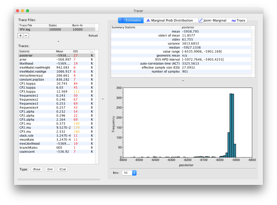
On the left hand side at the top is the name of the log file loaded (in this case YFB.log), the number of states in the log and the burn-in (10% by default). Below this is a table containing all the columns in the log file, including various statistics and continuous parameters. Selecting a trace on the left brings up analyses for this trace on the right hand side depending on the tab that is selected at the top. When first opened, the posterior trace (a quantity proportional to posterior — the product of the data likelihood and the prior probabilities, on the log-scale) is selected and various statistics of this trace are shown under the Estimates tab.
In the top right of the window is a table of calculated statistics for the selected trace. The statistics and their meaning are described in the table below.
- mean
- The mean value of the samples.
- stderr of mean
- The standard error of the mean. This takes into account the effective sample size so a small ESS will give a large standard error.
- stdev
- The standard deviation of the samples.
- variance
- The variance of the samples.
- median
- The median value of the samples.
- value range
- The full range of values sampled.
- geometric mean
- The central tendency or typical value of the set of samples.
- 95% HPD Interval
- The lower bound and upper bound of the highest posterior density (HPD) interval. The HPD is the shortest interval that contains 95% of the sampled values.
- auto-correlation time (ACT)
- The average number of states in the MCMC chain that two samples have to be separated by for them to be uncorrelated (i.e. independent samples from the posterior). The ACT is estimated from the samples in the trace (excluding the burn-in).
- effective sample size (ESS)
- The effective sample size (ESS) is the number of independent samples that the trace is equivalent to. This is calculated as the chain length (excluding the burn-in) divided by the ACT.
- number of samples
- The number of samples (values) used to compute the above statistics. This will be the total number of samples minus the burn-in.
Note that the effective sample sizes (ESSs) for all the traces are small (ESSs less than 100 are highlighted in red by Tracer and values > 100 but < 200 are in yellow). This is not good. A low ESS means that the trace contained a lot of correlated samples and thus may not represent the posterior distribution well. In the bottom right of the window is a frequency plot of the samples which is expected given the low ESSs is extremely rough.
If we select the tab on the right-hand-side labelled Trace we can view the raw trace, that is, the sampled values against the step in the MCMC chain:
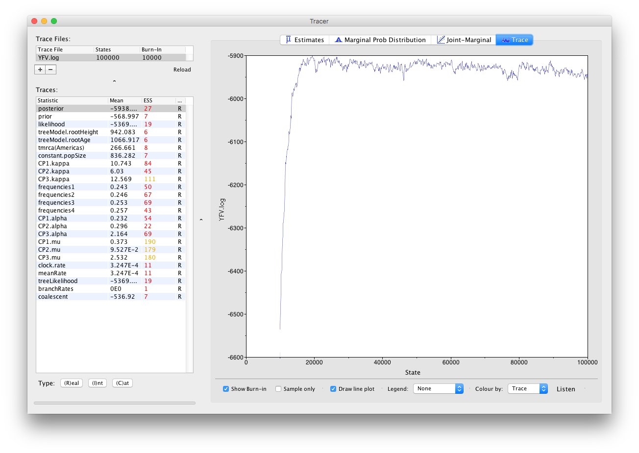
Here you can see how the samples are autocorrelated — there are 1000 samples in the trace (we ran the MCMC for 100,000 steps sampling every 100) but it is clear that adjacent samples often tend to have similar values. The ESS for the age of the root (age(root)) is only about 4 so we are only getting 1 independent sample to every 250 actual samples).
It also seems that the default burn-in of 10% of the chain length is inadequate (the posterior values are still increasing over most of the chain). Not excluding enough of the start of the chain as burn-in will bias the results and render estimates of ESS unreliable. Set the burn-in to 20,000 (doule-click on the number in the trace file table to edit it). You should see something like this:
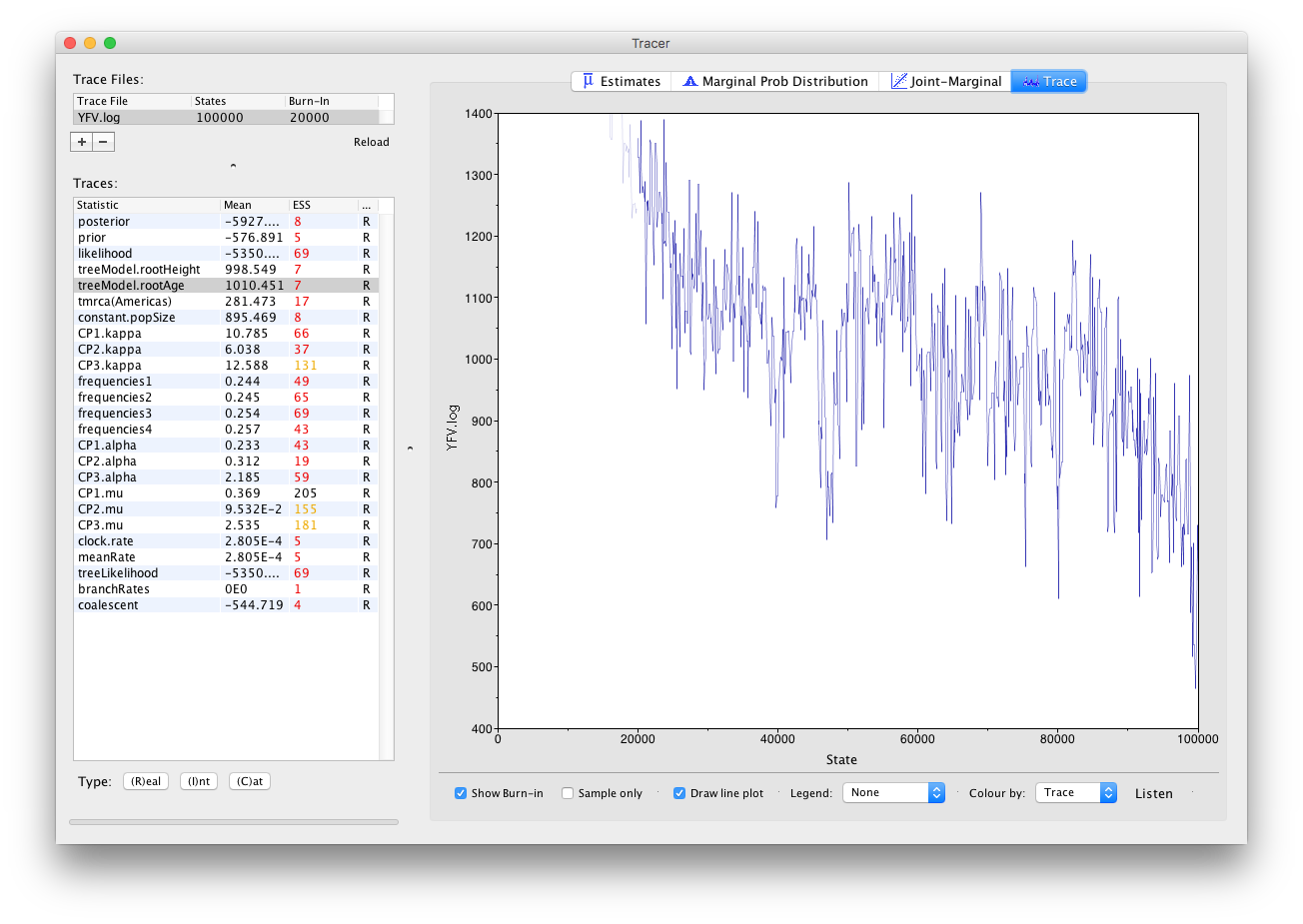
You may see some improvement in the ESSs but they will still be very low. In the image above, the root age looks to have a trend downwards which may mean that it hasn’t burnt-in yet or it may be part of a longer cycle of autocorrelated values.
The simple response to this situation is that we need to run the chain for longer. Go back to BEAUti (which hopefully you left open), go to the MCMC options section, above, and create a new BEAST XML file with a longer chain length (e.g. 10,000,000).
Import the new longer log file for the strict clock run, select the age(root) statistic and click on the Trace tab to look at the raw trace plot.
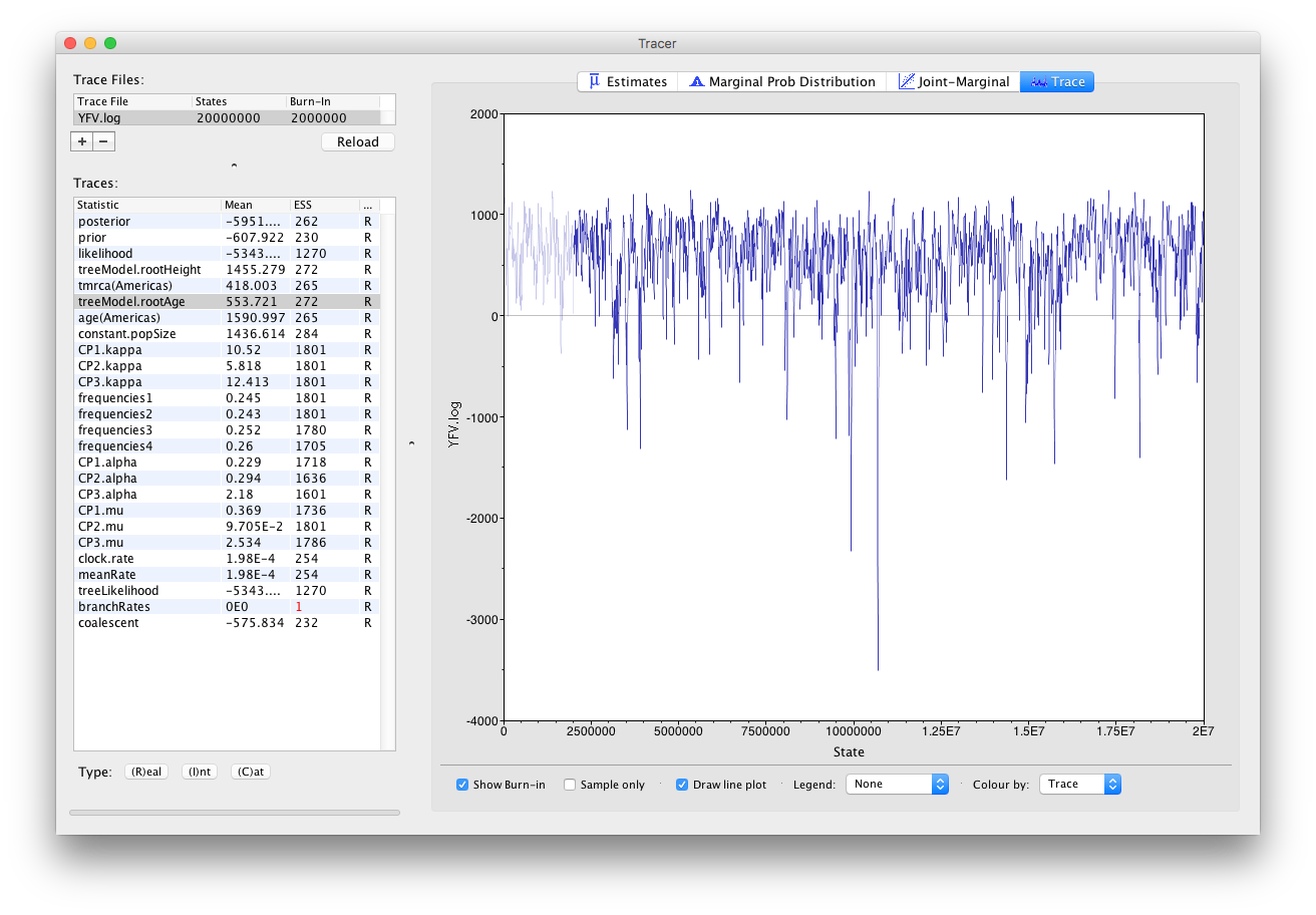
The log file provided contains 2000 samples and with an ESS of 310 for the clock.rate there is still some degree of auto-correlation between the samples but 310 effectively independent samples will now provide an reasonable estimate of the posterior distribution. There are no obvious trends in the plot which would suggest that the MCMC has not yet converged, and there are no large-scale fluctuations in the trace which would suggest poor mixing.
As we are happy with the behavior of posterior probability we can now move on to one of the parameters of interest: substitution rate. Select clock.rate in the left-hand table. This is the average substitution rate across all sites in the alignment. Now choose the density plot by selecting the tab labeled Marginal Prob Distribution. This plot shows a kernel density estimate (KDE) of the posterior probability density of this parameter. You should see a plot similar to this:
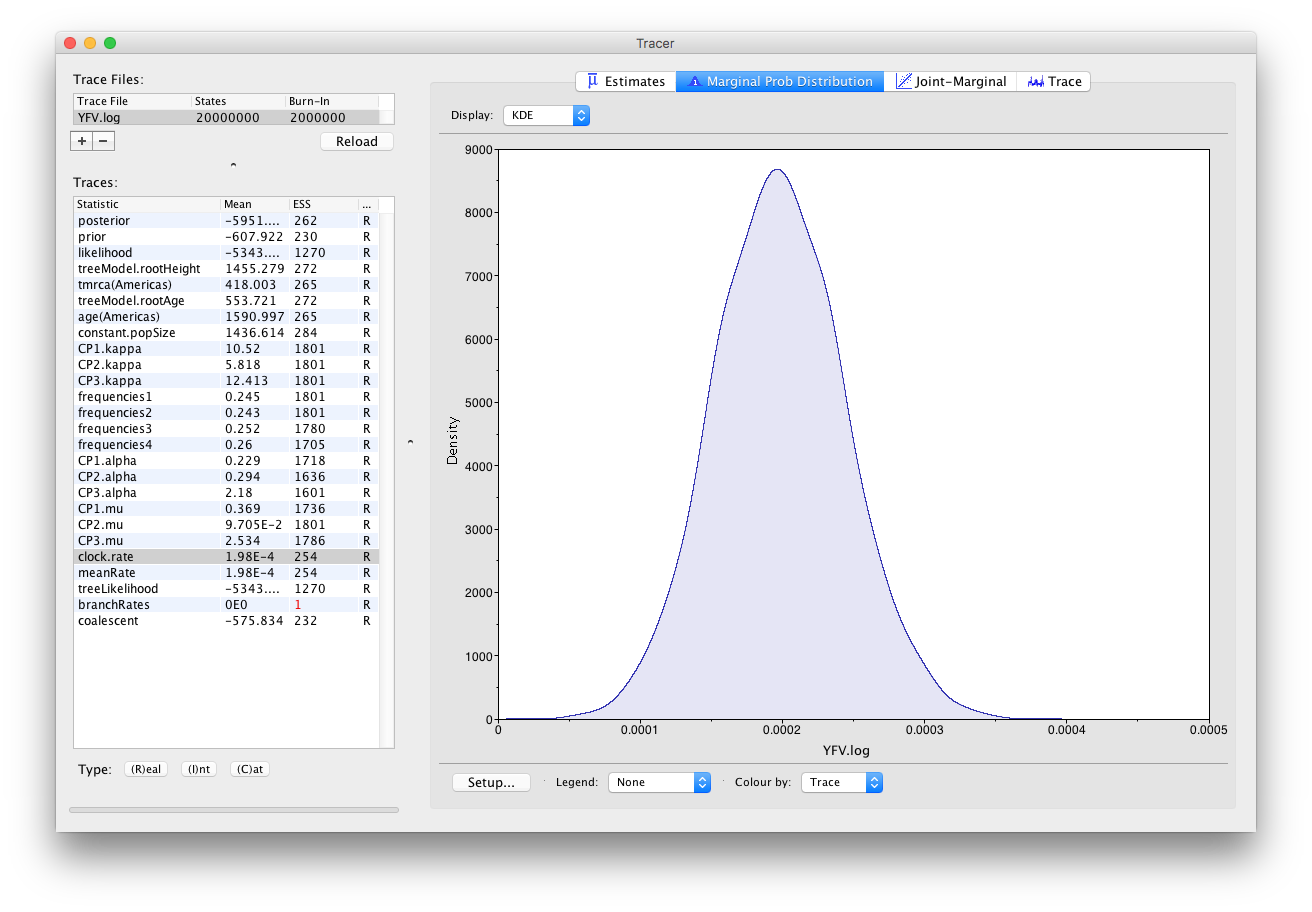
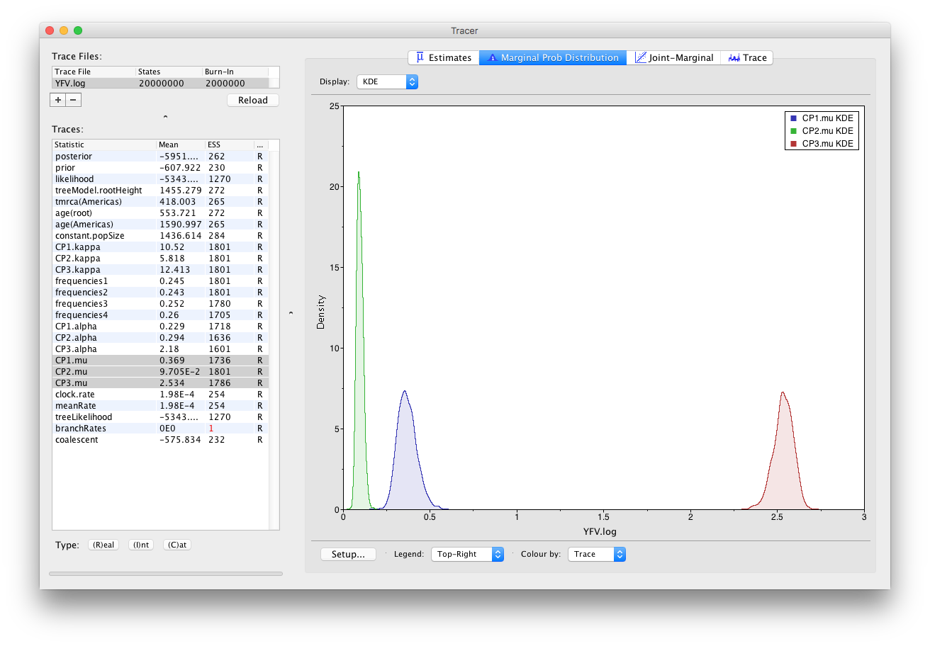
As you can see the posterior probability density is nicely bell-shaped. When looking at the equivalent histogram in the Estimates panel, there is some sampling noise which is smoothened by the KDE; this would be reduced if we ran the chain for longer but we already have a reasonable estimate of the mean and HPD interval. You can overlay the density plots of multiple traces in order to compare them (it is up to the user to determine whether they are comparable on the the same axis or not). Select the relative substitution rates for all three codon positions in the table to the left (labelled CP1.mu, CP2.mu and CP3.mu). This will show the posterior probability densities for the relative substitution rate at all three codon positions overlaid:
Now, let’s have a look at the timescale of the tree. Select the statistics called age(root) and age(Americas). These are the dates of the root of the tree and the clade we defined for all of the American sequences. Because we have dated the tips of the tree, these statistics are given as the calendar year with the present day being on the right hand side (the most recently sampled sequence is from 2009).
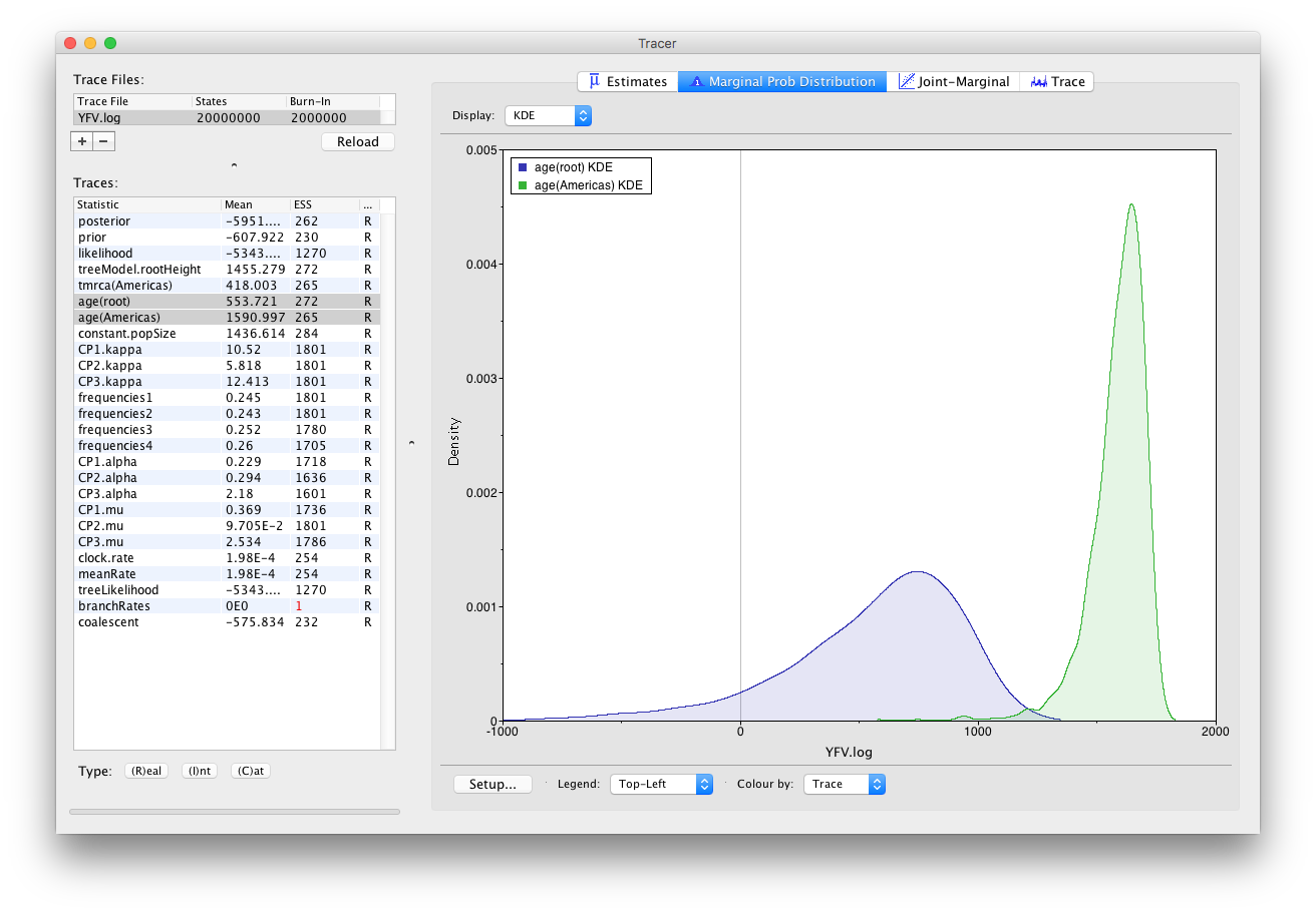
This indicates that the TMRCA for the Americas is significantly more recent than the entire tree and argues for a relatively recent introduction of yellow fever virus into the Americas. Note, however, that there is considerable uncertainty in these estimates. Switching to the Estimates panel shows that the mean date of of the TMRCA into the Americas is the year 1635 but the 95% HPD credible interval spans 1493 to 1765. Bryant et al. (2007) suggest that the introduction of YFV into the Americas is likely the result of the Atlantic slave trade which occurred from the 16th to 19th Centuries.
Summarizing the trees
We have seen how we can diagnose our MCMC run using Tracer and produce estimates of the marginal posterior distributions of parameters of our model. However, BEAST also samples trees (either phylogenies or genealogies) at the same time as the other parameters of the model. These are written to a separate file called the YFV.trees file. This file is a standard NEXUS format file. As such it can easily be loaded into other software in order to examine the trees it contains. One possibility is to load the trees into a program such as PAUP* and construct a consensus tree in a similar manner to summarizing a set of bootstrap trees. In this case, the support values reported for the resolved nodes in the consensus tree will be the posterior probability of those clades.
In this tutorial, however, we are going to use a tool that is provided as part of the BEAST package to summarize the information contained within our sampled trees.
Once running, you will be presented with a window like the one below:
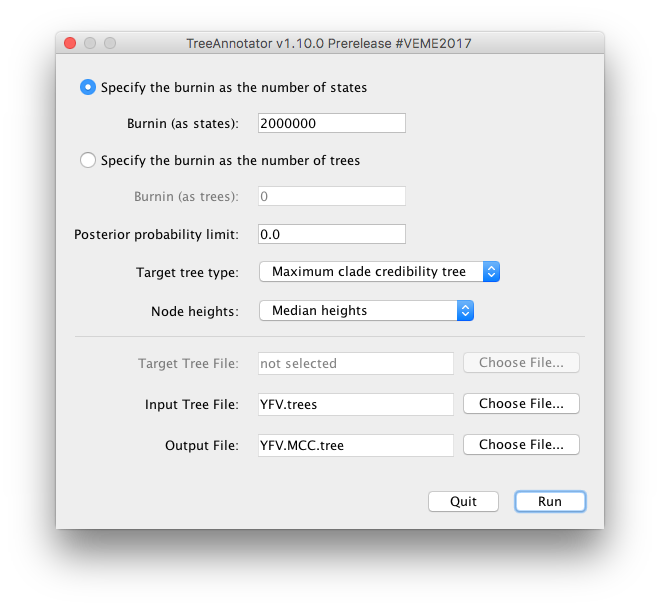
TreeAnnotator takes a single target tree and annotates it with the summarized information from the entire sample of trees. The summarized information includes the average node ages (along with the HPD intervals), the posterior support and the average rate of evolution on each branch (for models where this can vary). The program calculates these values for each node or clade observed in the specified ‘target’ tree.
- Burnin
- This is either the number of states or the number of trees in the input file that should be excluded from the summarization. This value is given as the number of trees rather than the number of steps in the MCMC chain. For the example, with a chain of 20,000,000 steps, a burn-in of 10% as the number of states can be specified as 2,000,000 states. Alternatively, if sampling every 10000 steps, there are 2000 trees in the file. To obtain a 10% burnin, set the burnin as the number of trees value to 200.
- Posterior probability limit
- This is the minimum posterior probability for a node in order for TreeAnnotator to store the annotated information. I.e., a value of 0.5 will mean that only nodes in the MCC tree that are present in at least 50% of the posterior distribution of trees will have posterior probabilities, height HPDs etc.
- Target tree type
- This has two options “Maximum clade credibility” or “User target tree”. For the latter option, a NEXUS tree file can be specified as the Target Tree File, below. For the former option, TreeAnnotator will examine every tree in the Input Tree File and select the tree that has the highest product of the posterior probabilities of all its nodes.
- Node heights
- This option specifies what node heights (times) should be used for the output tree. If the ’Keep target heights’ is selected, then the node heights will be the same as the target tree. Node heights can also be summarised as a Mean or a Median over the sample of trees. Sometimes a mean or median height for a node may actually be higher than the mean or median height of its parental node (because particular ancestral-descendent relationships in the MCC tree may still be different compared to a large number of other tree sampled). This will result in artifactual negative branch lengths, but can be avoided by the ‘Common Ancestor heights’ option.
- Target Tree File
- If the “User target tree” option is selected then you can use “Choose File…” to select a NEXUS file containing the target tree.
- Input Tree File
- Use the “Choose File…” button to select an input trees file. This will be the trees file produced by BEAST. Output File - Select a name for the output tree file.
Select a Burnin (as states) of 2,000,000, Posterior probability limit of 0.0, Target tree type: Maximum clade credibility tree, and Node heights: Median heights. Then select YFV.trees as the Input Tree File.
Once you have selected all the options above, press the Run button. TreeAnnotator will analyze the input tree file and write the summary tree to the file you specified. This tree is in standard NEXUS tree file format so may be loaded into any tree drawing package that supports this. However, it also contains additional information that can only be displayed using the FigTree program.
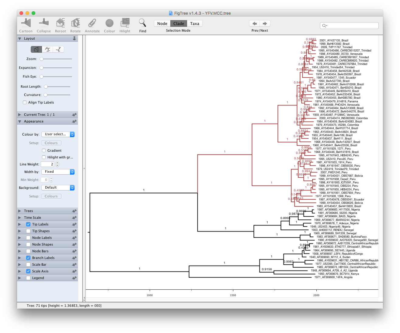
Viewing the annotated tree
Run FigTree now and select the Open... command from the File menu. Select the tree file you created using TreeAnnotator in the previous section. The tree will be displayed in the FigTree window. On the left hand side of the window are the options and settings which control how the tree is displayed. In this case we want to display the posterior probabilities of each of the clades present in the tree and estimates of the age of each node. In order to do this you need to change some of the settings.
First, re-order the node order by Increasing Node Order under the Tree menu. Click on Branch Labels in the control panel on the left and open its section by clicking on the arrow on the left. Now select posterior under the Display: option.
We can also plot a time scale axis for this evolutionary history: select Scale Axis and deselect Scale bar. By default the timescale is going forwards in time from the root of the tree. For appropriate scaling, set the Reverse Axis option in the Scale Axis panel and open the Time Scale section of the control panel setting the Offset to 2009.0.
Finally, open the Appearance panel and alter the Line Weight to draw the tree with thicker lines. You can also color clades by selecting a branch, select the Clade selection mode and choose a color. None of the options actually alter the tree’s topology or branch lengths in anyway so feel free to explore the options and settings (Highlight or Collapse the Americas clade, for example ).
You can also save the tree and this will save most of your settings so that when you load it into FigTree again it will be displayed almost exactly as you selected.
Finally, the tree can also be exported to a graphics file (pdf, svg, etc.) using the options in the File menu.
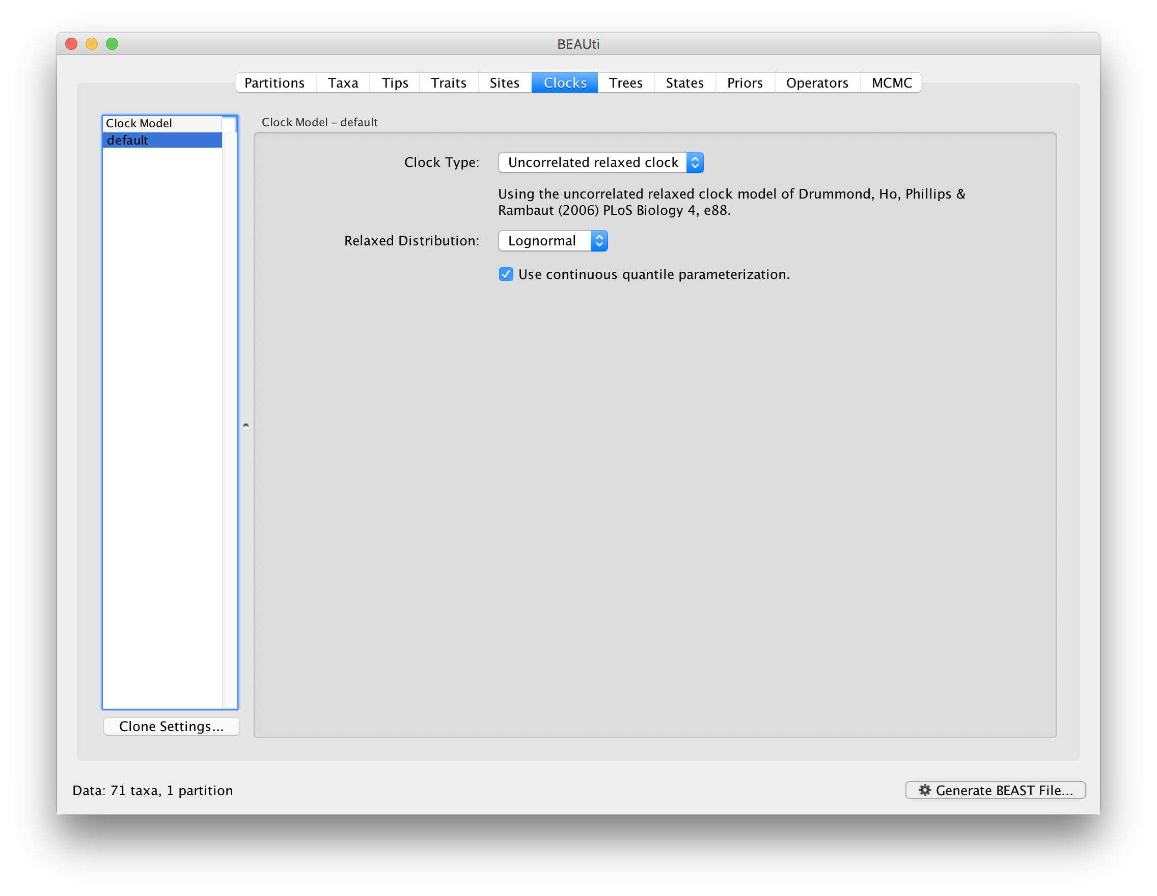
Relaxed molecular clock analysis
A relaxed clock analysis using a lognormal distribution can also be set up for this data set, by selecting the relevant clock model in the Clocks tab:
Also for this analysis, we made available the output files for a longer run:
References
Bryant JE, Holmes EC and Barrett ADT (2007) Out of Africa: A Molecular Perspective on the Introduction of Yellow Fever Virus into the Americas. PLoS Pathogens, 3: e75. doi: 10.1371/journal.ppat.0030075
Help and documentation
The BEAST website: http://beast.community
Tutorials: http://beast.community/tutorials
Frequently asked questions: http://beast.community/faq