Construct a model in BEAUti | BEAST Documentation

This page discusses how to construct a phylogenetic model for your data using the graphical user interface in BEAUti. It describes how to link and unlink model components for different data partitions (such as substitution models or molecular clock models). It also discusses linking individual parameters for even more flexibility.

Written by: Andrew Rambaut

Last updated: August 12, 2017

Data partitions are the basic unit of data in BEAST. They are a collection of sequence data (DNA, amino acid or other), discrete traits, or continuous traits for each of a set of taxa that are connected by a tree and are assumed to have a shared evolutionary process. Each data partition has a tree, a site model, and a molecular clock model. Data partitions can share these models (their models are linked) or have their own models (their models are unlinked). You can link and unlink these model components in the Partitions panel of BEAUti — see Linking and unlinking models, below. Even if partitions have unlinked model components, individual parameters of the models can be linked either directly — see Linking parameters — or as a hierarchical phylogenetic model (HPM) — see Hierarchical phylogenetic models, below and this tutorial.

Importing data partitions

To load a sequence alignment, select the Import Data... option from the File menu. You can also click the + button at the bottom left of the window or just drag-and-drop the file into the main window. The data should be in either NEXUS or FASTA format. BEAUti will also import the data from a BEAST XML file (including all the data partitions, the dates of the tips, but not the models and settings).

Importing partitions from a NEXUS file

NEXUS files can define multiple partitions using the charset command. For example, the example file in the BEAST package: /examples/Data/H1N1_HA.nex (or download from here) divides the sequences into two partitions (note the sequences have been truncated here for brevity):

#NEXUS

BEGIN DATA;
	DIMENSIONS NTAX=25 NCHAR=1695;
	FORMAT MISSING=? GAP=- DATATYPE=DNA;
	MATRIX
hSCar1918     ATGGAGGCAAGACTACTGGTCTTGTTATGTGCATTTGCA...
hCambr39      ATGAAGGCAAGACTACTGGTCCTGTTATGTACACTTGCA...
hCHR83        ATGAAAGCAAAACTACTGGTCCTGTTATGTGCACTCTCA...
hFortMon47    ATGAAAGCAAAACTACTGATCCTGTTATGTGCACTTACA...
hKiev79       ATGAAAGCAAAACTACTGGTCCTGTTATGTGCACTTTCA...
hLenin54      ATGAAAGCAAAACTACTGGTCCTGTTATGTGCACTTTCA...
hMongol85     ATGAAAGCAAAACTACTGGTCCTGTTATGTGCACTTTCA...
hMongol91     -----------CCTAGTGGTCCTGTTATGTGCATTTACA...
hNWS33        ATGAAGGCAAAACTACTGGTCCTGTTATGTGCACTTGCA...
hPR34         ATGAAGGCAAACCTACTGGTCCTGTTATGTGCACTTGCA...
hScot94       ATGAAAGAAAAACTACTGGTCCTGTTATGTGCACTTTCA...
hSuita89      ATGAAAGCAAAACTACTAGTCCTGTTATGTGCATTTACA...
hUSSR77       ATGAAAGCAAAACTACTGGTCCTGTTATGTGCACTTGCA...
sEhime80      ATGAAGGCAATACTATTAGTCTTGCTATGTACATTTGCA...
sIllino63     ATGAAGGCAATACTATTAGTCTTGTTATGTGCATTTGCA...
sIowa30       ATGAAGGCAATACTATTAGTCTTGTTATGTGCATTTGCA...
sNebrask92    ATGAAGGCAATACCATTAGTCTTGCTATATACATTTACA...
sNewJers76    ATGAAGGCAATACTATTAGTCTTGTTATGTACATTTGCA...
sStHya91      ATGAAAGCAATACTATTAGTCTTGCTATATACATTTACA...
sWiscons61    ATGAAGGCAATACTATTAGTCTTGTTATGTGCATTTGCA...
sWiscons98    ATGAAGGCAATACTATTAGTCTTGCTATATACATTCACA...
aDuckA76      ATGGAAGCAAAACTATTTGTACTATTCTGTACATTCACT...
aDuckB77      ATGGAAGTAAAACTATTTGTATTATTCTGCACATTCACT...
aItaly87      ATGGAAGCAAAACTGTTTGTATTATTCTGTACATTCACT...
aMallard85    ATGGAAGTAAAACTATTTGTACTATTCTGTACATTCACT...
;
END;

begin assumptions;
	charset HA1 = 151-920;
	charset HA2 = 1-150,921-1695;
end;

This alignment comprises haemagglutinin (HA) gene sequences from a collection of influenza viruses (the letter at the beginning of the labels denotes the host; a = avian, s = swine and h = human). The file contains two charset commands which define two domains of the protein — HA1, the globular domain and HA2, the stem region. Note the HA1 domain lies within the HA2 so the latter is defined as two regions which are concatinated.

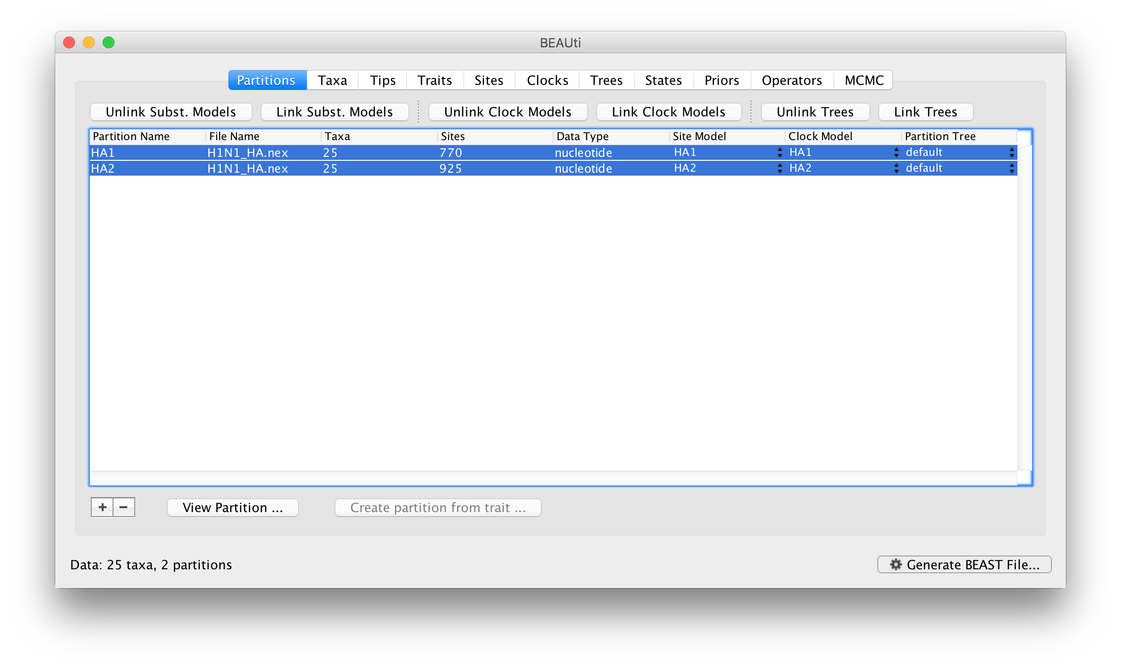
When imported into BEAUti this results in two partitions in the Partitions panel:

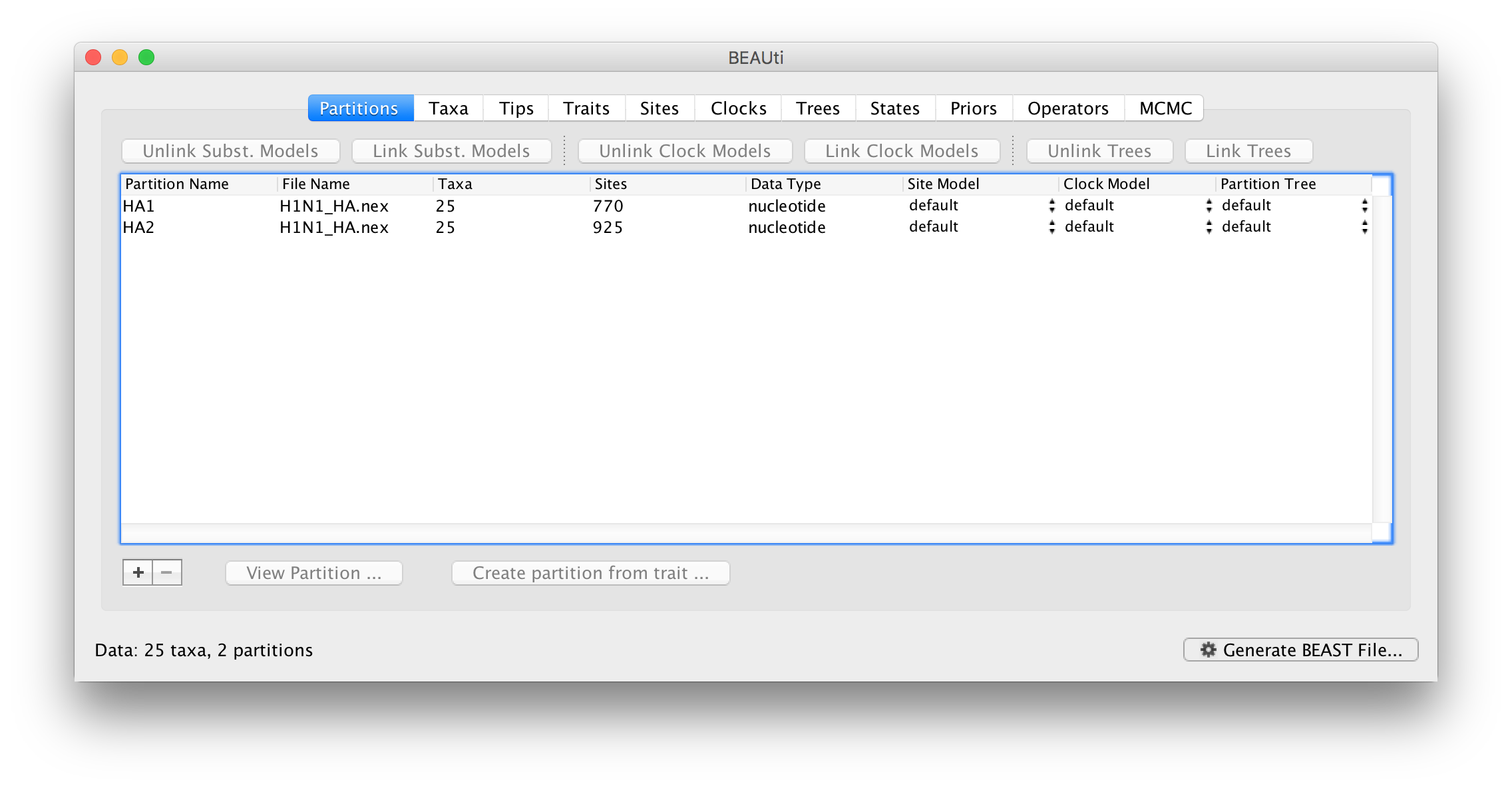
The two partitions by default share the same substitution model, clock model and tree. You can see that the Site model, Clock model and Partition tree columns of the table are defined as default.

Importing partitions from multiple files

The other way to load multiple partitions is simply to import them from different alignment files (NEXUS, FASTA or XML). The partitions will appear in the table named after the file they were loaded from. In most cases you should load partitions with exactly the same set of taxa (the names should be identical). If the partitions’ set of taxa differ in any way from each other then BEAUti will give them a different clock model and partition tree.

Tip dates

The first thing to do is to specify the dates of sampling of the sequences using the Tips panel. The year that each virus was isolate is given at the end of the labels. To extract the dates select the Use tip dates box and click the Parse Dates button and in the dialog box choose the Defined just by its order, Order: last, and Parse as a number options. See this page for more details of how to use this dialog box to parse dates from tip labels.

Site models

Site models specify the evolutionary process that describes how the data was generated on the tree. For example, for DNA sequences this could be an HKY model with discrete gamma rate heterogeneity amongst sites. If you switch to the Sites panel using the tabs at the top, you can specify the details of this model.

On the left hand side is a table listing the site models currently in use. At the moment it only has the default which is being shared by both the data partitions:

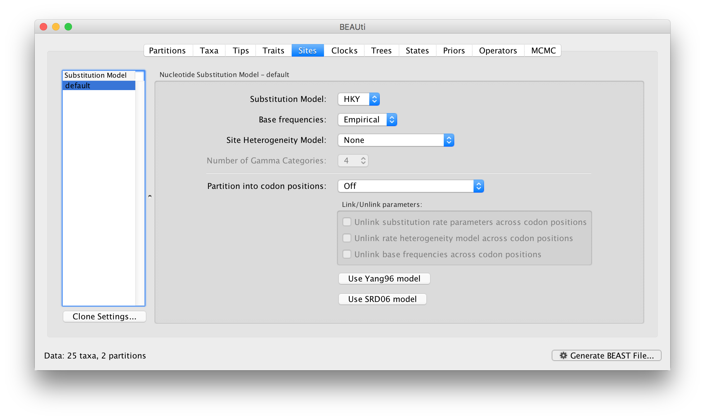
The model settings on the right are for this site model. The default is the HKY model which has a parameter, kappa, specifying the ratio of transition and transversion rates.

Molecular clock models

Switch to the Clocks panel to set the clock model settings. In the same way as before, the current clock models are given in the table on the left and the settings for them on the right. Select the Uncorrelated relaxed clock as the choice for default:

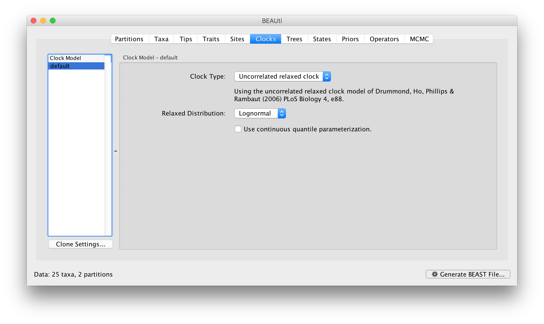
For the log normal model has two parameters, ucld.mean and ucld.stdev which are the mean and standard deviation of the lognormal distribution describing the distribution of rates on the branches in the tree. See this page for more details about the various clock models and their parameters.

Tree priors

In the Trees panel we again see the available trees on the left and the settings on the right. In this case the settings for the tree are actually the choice of tree prior:

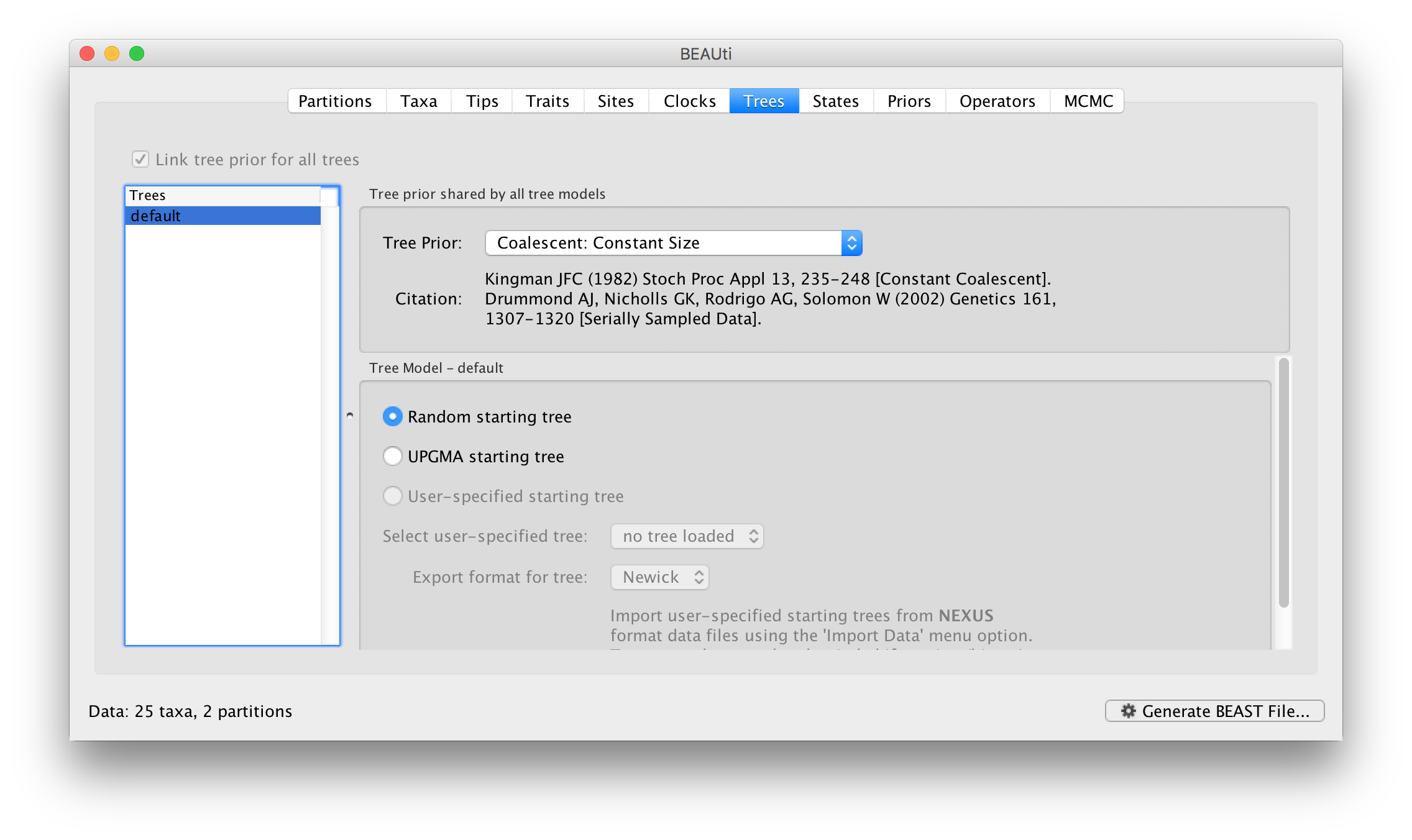
The different tree priors available are described in more detail here.. For this, leave it at the default, Coalescent: Constant Size.

Linking and unlinking models

We will now look at linking and unlinking the components of the model to constuct different scenarios for the evolution of these sequences.

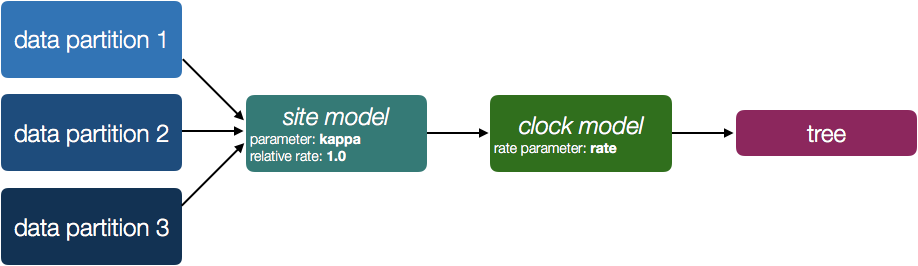
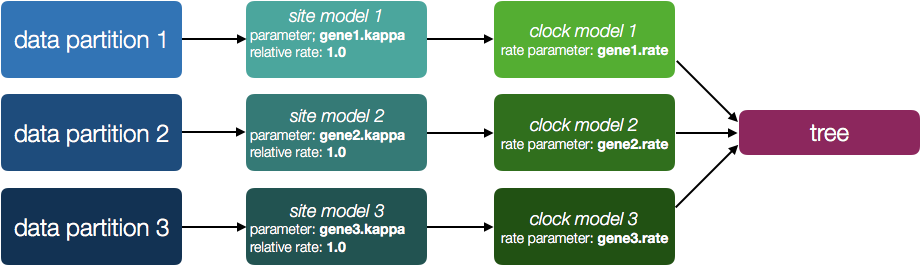
To start with all the partitions share the same site model, molecular clock model and tree. So this is saying that all the sites in both partitions are evolving in the same way, at the same rate and on the same tree (Figure 1).

**Figure 1** | All partitions sharing the same site model, molecular clock model and tree. The parameters of these components are estimated across all data partitions.

Unlinking site models

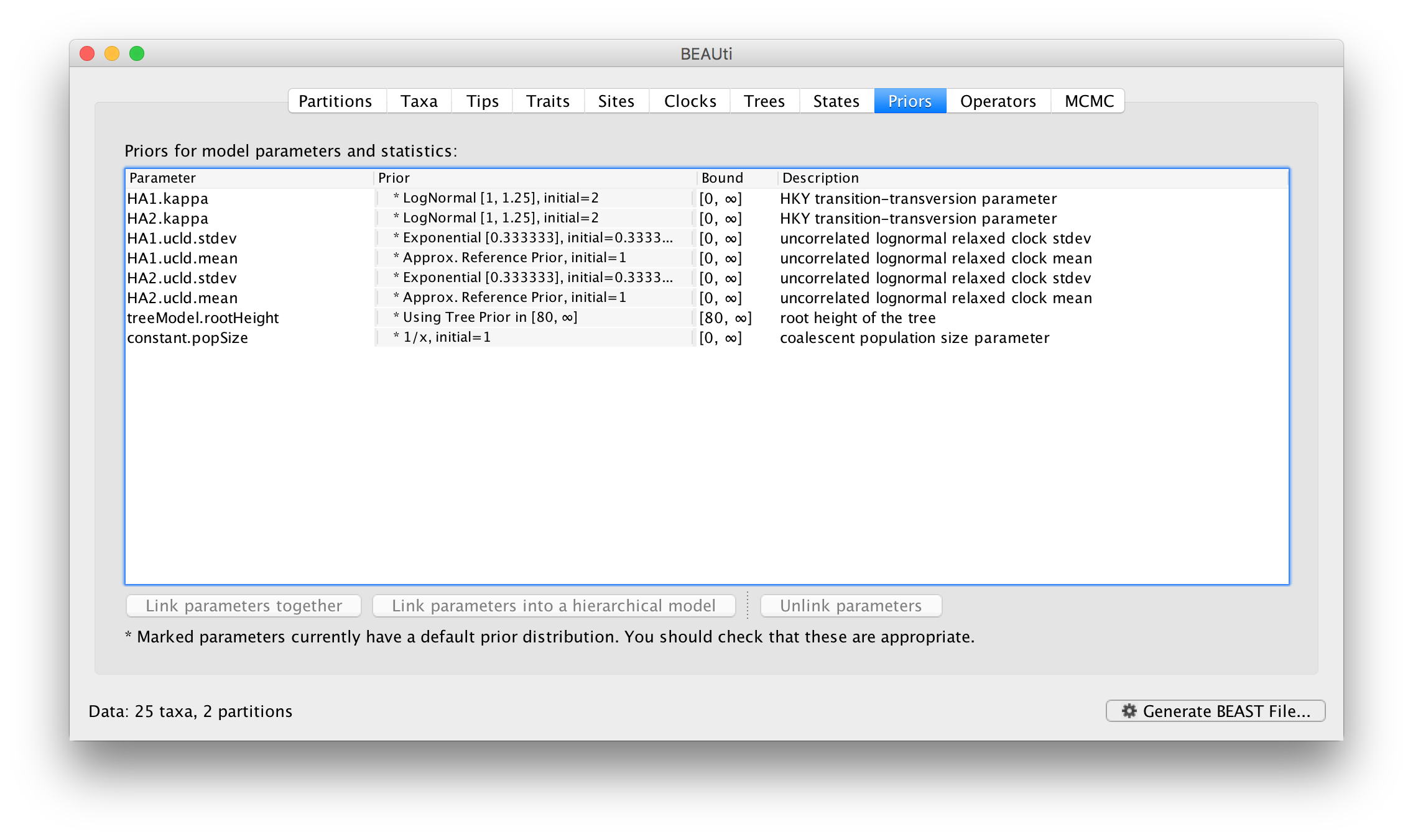
As it stands this means the model specified is as if a single partition with all the data had been imported. To relax this model, we can return to the Paritions panel. Select both partitions in the table and click the Unlink Subst. Models button. The result is that each partition gets its own site model (named after the partition):

The settings for the two new site models will be copied from the existing ‘default’ one but now there will be a separate kappa parameter for each. In the Priors panel you will now see HA1.kappa and HA2.kappa:

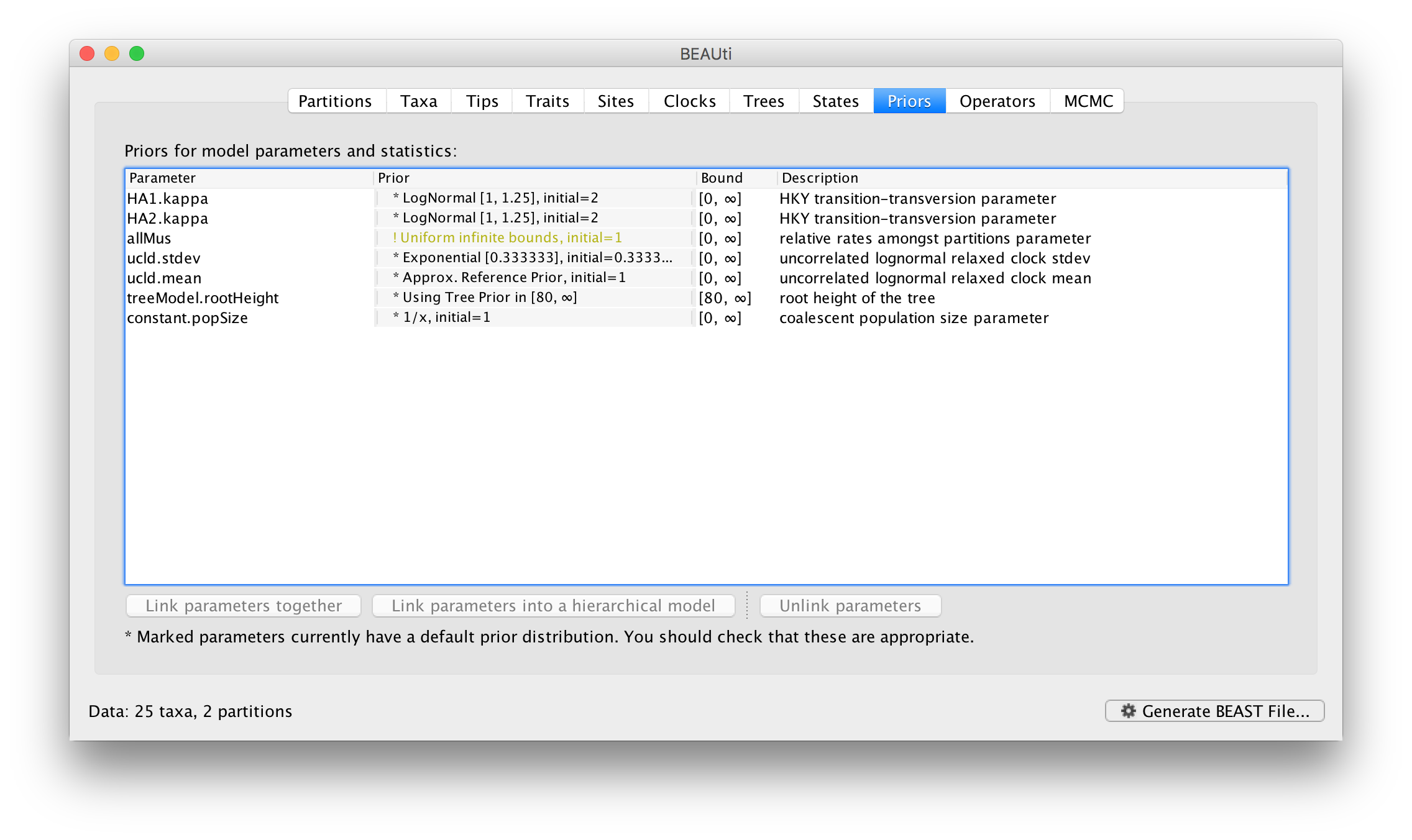
You will also see a new parameter, allMus which is a vector of relative rates, one for each partition. These are constrained to have a mean of 1.0 and are multiplied by the overall molecular clock rate to get the rate for each partition. In this way the rate of evolution can vary between data partition but because they share the same clock model the relative rate on each branch of the tree is the same. A general diagram of the scenario is shown in Figure 2.

**Figure 2** | The partitions each have their own site model, kappa parameter, and relative rate mu, but share a single molecular clock model and tree. This construction implies that whatever evolutionary forces or constraints are controlling the rates of evolution (and the details of the substitution process represented by kappa) differ between the data partitions. The relaxed clock also allows the rates to vary from branch to branch but this variation is shared between all partitions --- an extrinsic factor that operates on the whole genome.

Unlinking clock models

Select both partitions in the data partition table and click the Unlink Clock Models button. The result is that each partition gets its own clock model (again, named after the partition):

Returning to the Priors panel, you will notice some changes:

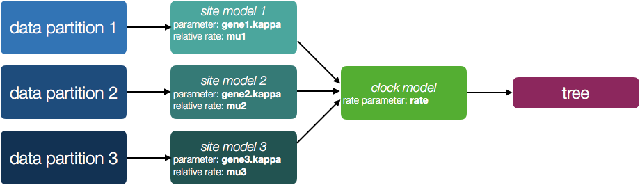
The allMus parameter has been removed and replaced with a ucld.mean and ucld.stdev for each partition. This is because each partition now has its own molecular clock with its own independent rate so not longer needs a relative rate. Each partition also has its own distribution from which the relative rates for each branch are drawn (again, independently for each partition). A general diagram is shown in Figure 3.

**Figure 3** | The partitions each have their own site model, kappa parameter, molecular clock model, rate parameter but still share the tree. This model implies that not only do the evolutionary forces or constraints vary between the data partitions but that these forces also vary from branch to branch independently for each partition.

Codon partitions

Data partitions comprising protein-coding nucleotide sequences can be subdivided into codon position partitions. This is done in the Sites panel:

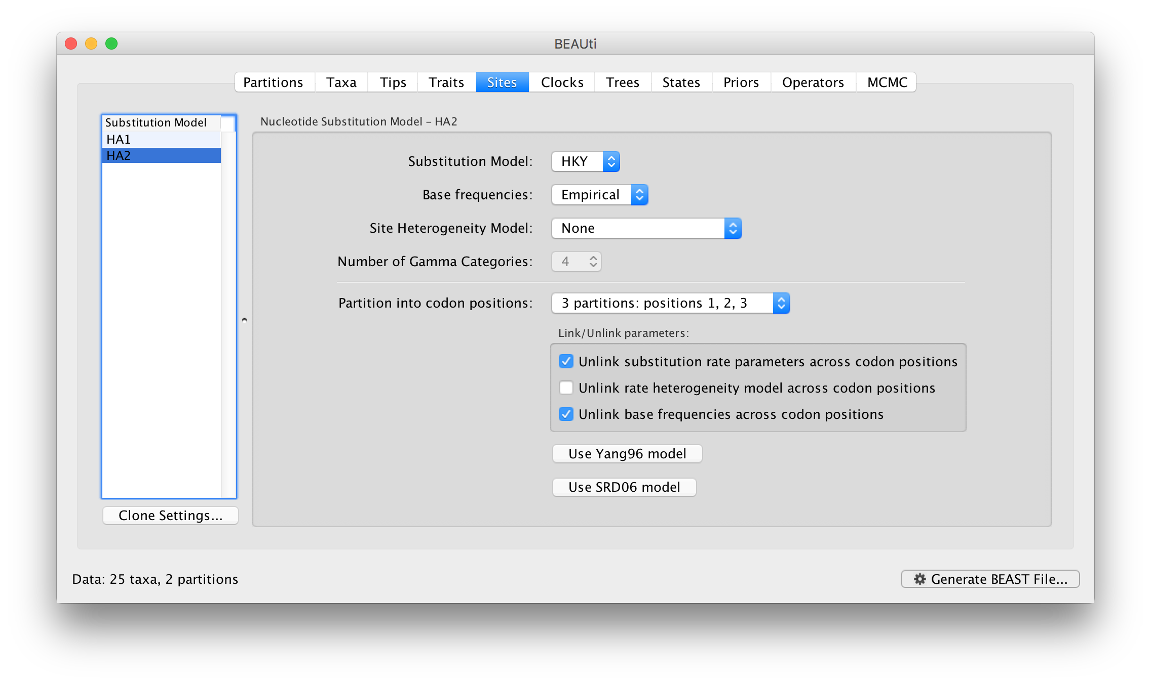
Select the HA1 partition and then select from the Partition into codon positions menu. Select 3 partitions: positions 1, 2, 3. Do the same for the HA2 partition. In the Priors panel you will see that each of the 3 codon positions for each of the partitions now has its own kappa parameter (HA1.CP1.kappa is the kappa for theHA1 partition, codon position 1, etc.):

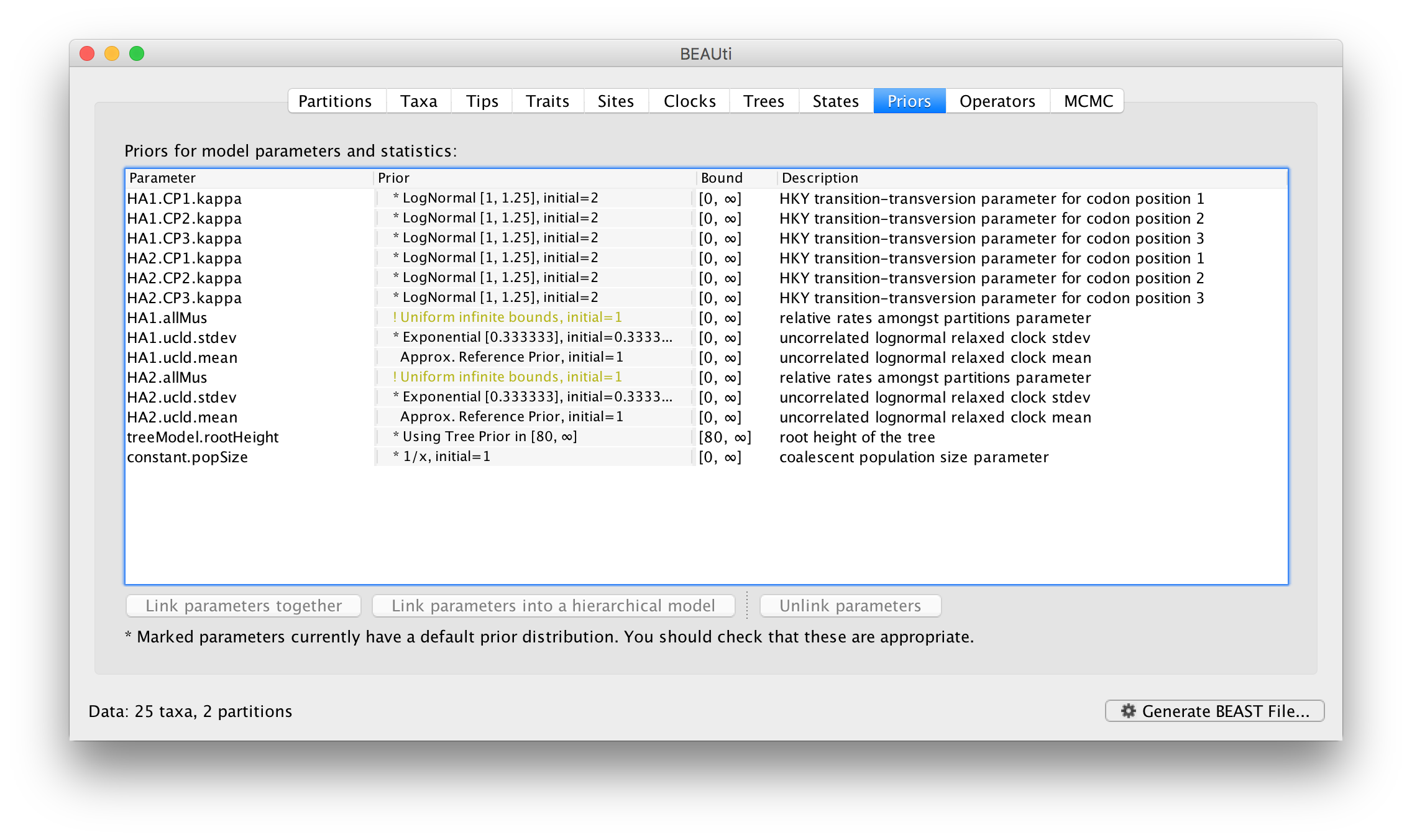
You will also that each partition now has its own allMu vector parameter. These are the set of relative rates for the codon positions for each partition. This is the equivalent of compiling each of the first, second, and third codon positions for each gene region into separate partitions but is generally more convenient. The codon positions of a particular partition share the same clock model and substitution model but this is probably the appropriate assumption.

Linking parameters

At this stage we have a very general, parameter rich, model and we may wish to constrain it by linking particular parameters. This links two or more independent parameters that they are a single entity that always have the same value. This allows you to jointly estimate the parameter across different partitions even though other aspects of their models are independent. For example, we can link the overall rate of evolution for our two partitions. In the Priors select the two clock rate parameters (HA1.ucld.mean and HA2.ucld.mean) and click the Link parameters together button. A dialog box will appear showing the parameters being linked, the name of the new ‘controlling’ parameter and the prior on this parameter:

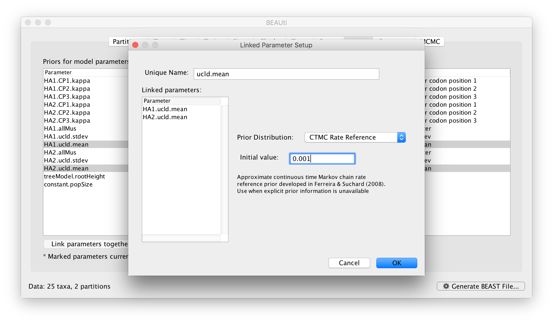
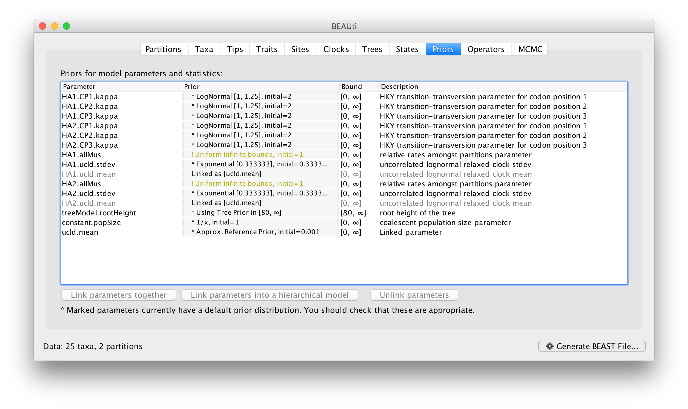
Name the new parameter but leave the other options at their defaults, click OK and you see the table has been updated so the linked parameters are in grey and the new controlling parameter is at the bottom:

You could also link the HA1.ucld.stdev and HA2.ucld.stdev parameters similarly. Linking both the ucld.mean and ucld.stdev parameters of the clock models for the two partitions together is saying that the rates of evolution for each branch is drawn from exactly the same distribution for each partition, but which actual branch is a fast or slow one is different.

Or you could link HA1.CP1.kappa with HA2.CP1.kappa, and HA1.CP2.kappa with HA2.CP2.kappa, etc. This would say that codon position 1 in ‘HA1’ has the same underlying ratio of transitions to tranversions as ‘HA2’ even if the rates differ between them.

Hierarchical phylogenetic models

You can also link parameters together in a Hierarchical phylogenetic model (HPM). This takes the approach that the individual parameters are not exactly the same but rather are drawn from a common underlying distribution (say a normal distribution) and the parameters of that distribution (the mean and stdev for the normal) are then estimated. For more information about HPMs see this tutorial.

Unlinking trees

The ultimate, most general, model is to also unlink the trees between partitions (using the Unlink Trees button in the Partitions panel). Doing this results in each partition not only have its own subtitution model, molecular clock model and parameters but also a completely different tree. Just doing this essentially performs independent analyses in a single BEAST run (probably not the most efficient way of doing this).

However there are a number of situations for which unlinking the trees may be appropriate. If the different partitions are independent, unlinked, loci from the same individuals then can be used in a multi-locus coalescent analysis to jointly estimate the demographic history.

If the data partitions are samples taken from different populations (i.e., viruses from separate outbreaks or from different patients) then they will, by definition, have different trees but parameter linking or hierarchical modelling could jointly estimate parameters which they do have in common (such as rate of evolution).

Tags: