Epoch Model Tutorial
This tutorial describes how to extend BEAST XML files, such as generated by BEAUti, to include analyses under time-heterogeneous (epoch) models (see Bielejec et al., 2014).
Introduction
In this tutorial we will show how to setup, run and analyse data with the epoch models described in Bielejec et al. (2014). We present an artificial example and describe the necessary steps to get an actual analysis up and running. Example files for this tutorial can be found here.
Prerequisites
This tutorial assumes that the user has a basic knowledge of the BEAST framework, knows how to generate an XML input file and can interpret basic output information of an MCMC run. BEAST runnables for all major platforms can be found here. You will need a Java runtime environment version 1.5 or greater to run the BEAST executable. Due to the computational intensity of the computations involved in the epoch model, the BEAGLE library also needs to be installed and used with the BEAST runs discussed here. See the BEAGLE website for details on how to install and use the BEAGLE library.
Data
Start by uploading your sequences into BEAUTi and generating a standard XML file. For simplicity we assume a single nucleotide partition in this example, a constant population size model and a strict molecular clock.
The data in this tutorial was artificially generated by evolving it on an MCC tree generated from a Bayesian phylogenetic analysis of human influenza A hemagglutinin gene sequences sampled through different epidemic seasons (Drummond and Suchard, 2010). This tree is visualised in Figure 1.
We will analyze the data with the HKY nucleotide substitution model (Hasegawa et al., 1985), focusing on estimating the κ parameter (i.e., the transition-transversion bias) in three separate epochs.
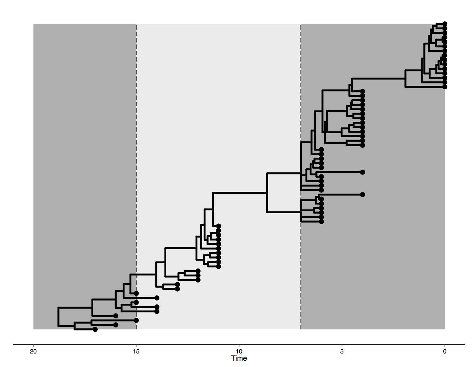
The first epoch lasts until transition time T1 set at 7 (i.e. 7 years before the most recent sampling date) and is governed by a model which we will call HKY1. The second epoch lies between transition times T1 and T2 = 15, with substitution model HKY2. Finally, everything past T2 occurs in a third epoch, with corresponding model HKY3.
Turning BEAST’s XML into an ‘epochized’ analysis
Open the file generated in the previous section in your favourite text editor. Scroll down to the block where the HKY model is defined. We need to define three separate models for each epoch, corresponding to HKY1, HKY2 and HKY3, therefore delete this block and paste there:
  <hkymodel id="hky.1">
    <frequencies>
      <frequencymodel idref="freqModel">
    </frequencymodel></frequencies>
    <kappa>
      <parameter id="kappa.1" lower="0.0" value="1.0">
    </parameter></kappa>
  </hkymodel>

  <hkymodel id="hky.2">
    <frequencies>
      <frequencymodel idref="freqModel">
    </frequencymodel></frequencies>
    <kappa>
      <parameter id="kappa.2" lower="0.0" value="1.0">
    </parameter></kappa>
  </hkymodel>

  <hkymodel id="hky.3">
    <frequencies>
      <frequencymodel idref="freqModel">
    </frequencymodel></frequencies>
    <kappa>
      <parameter id="kappa.3" lower="0.0" value="1.0">
    </parameter></kappa>
  </hkymodel>
The individual models that will make up the epoch model are now available, so we can now setup the epoch model itself. Below those three blocks paste:
 <epochBranchModel id="epochModel">
    <treeModel idref="treeModel"/>
    <epoch id="epoch1" transitionTime="10">
      <hkyModel idref="hky.1"/>
    </epoch>
    <epoch id="epoch2" transitionTime="15">
      <hkyModel idref="hky.2"/>
    </epoch>
    <hkyModel idref="hky.3"/>
 </epochBranchModel>
Each epoch block references its corresponding model and transition time that bounds it, with the last (i.e., the furthest in the past) model being unbounded. Now go to the line in the XML file where the site model is defined. We need to reference the epoch model we just defined as our substitution model of choice. Alter the corresponding line to have it look like this:
 <siteModel id="siteModel">
    <branchSubstitutionModel>
      <beagleSubstitutionEpochModel idref="epochModel"/>
    </branchSubstitutionModel>
 </siteModel>
Now go to the treeLikelihood block in the XML file. This block also needs to reference the epoch model. Change the corresponding line to read as follows:
 <treeLikelihood id="treeLikelihood">
    <patterns idref="patterns"/>
    <treeModel idref="treeModel"/>
    <siteModel idref="siteModel"/>
    <beagleSubstitutionEpochModel idref="epochModel"/>
    <strictClockBranchRates idref="branchRates"/>
 </treeLikelihood>
Since we now have three separate κ parameters, we need to define separate transition kernels and separate prior distributions for each of these parameters. Go to the operators block. Look for an operator which references kappa (our κ parameter). Delete this block and paste there:
  <scaleOperator scaleFactor="0.75" weight="0.1">
    <parameter idref="kappa.1"/>
  </scaleOperator>

  <scaleOperator scaleFactor="0.75" weight="0.1">
    <parameter idref="kappa.2"/>
  </scaleOperator>

  <scaleOperator scaleFactor="0.75" weight="0.1">
    <parameter idref="kappa.3"/>
  </scaleOperator>
All the other parameters in this analysis are shared, therefore there is no need to define separate transition kernels for them. Now look for the prior block, which you can find within the mcmc block. We need three prior distributions, one per each κ parameter (in this example we assume lognormally distributed κ parameters):
  <logNormalPrior mean="1.0" stdev="2" offset="0.0" meanInRealSpace="true">
    <parameter idref="kappa.1"/>
  </logNormalPrior>

  <logNormalPrior mean="1.0" stdev="2" offset="0.0" meanInRealSpace="true">
    <parameter idref="kappa.2"/>
  </logNormalPrior>

  <logNormalPrior mean="1.0" stdev="2" offset="0.0" meanInRealSpace="true">
    <parameter idref="kappa.3"/>
  </logNormalPrior>
Naturally we want to log the three parameters of our epoch model. To monitor the analysis we start with the screen log. Look for the following line:
<log id="screenLog" logEvery="5000">
Find the column block where the kappa parameter is referenced and paste these three blocks here instead:
  <column label="kappa.1" sf="6" width="12">
    <parameter idref="kappa.1"/>
  </column>

  <column label="kappa.2" sf="6" width="12">
    <parameter idref="kappa.2"/>
  </column>

  <column label="kappa.3" sf="6" width="12">
    <parameter idref="kappa.3"/>
  </column>
We then still need to modify the lines responsible for storing the parameter estimates of the epoch model to file. Go to the beginning of the log block responsible for keeping a log file, i.e.:
<log id="fileLog" logEvery="1000">
Find the line which references the κ parameter and paste there instead:
  <parameter idref="kappa.1"/>
  <parameter idref="kappa.2"/>
  <parameter idref="kappa.3"/>
We are done with editing the XML and can proceed to performing the analysis.
Performing the MCMC inference
Epoch model inference requires the BEAGLE library installed and configured to be visible for BEAST. Installation and setup of the BEAGLE library on various platforms is covered on this website.
In a UNIX/Linux environment, the XML edited in the previous section can be run from the command line using the following command:
java -Djava.library.path=/usr/local/lib -jar beast.jar epochExample.xml
Analyzing the output
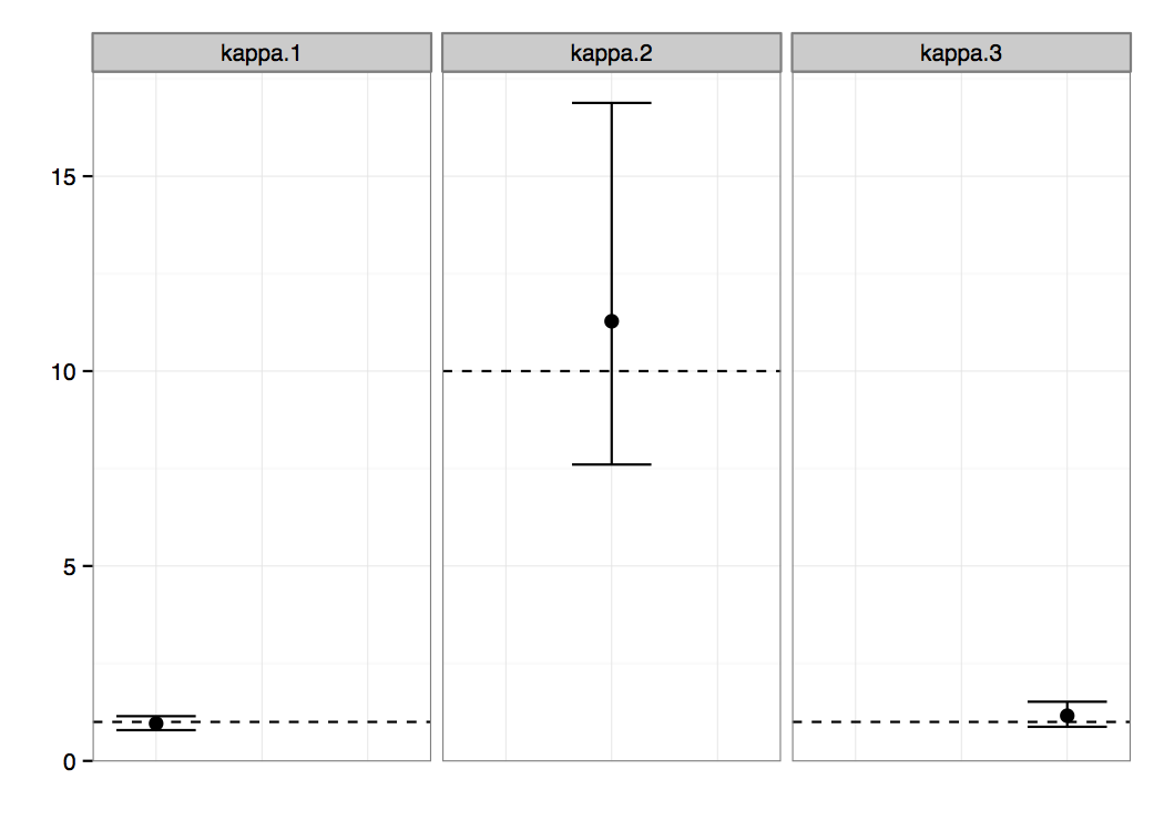
After the analysis has finished you can import the resulting log file into the software of your choice, e.g. Tracer (a program for analysing the trace files generated by MCMC runs. Figure 2 presents the posterior probability distributions of the κ parameters, which were our main interest in this analysis. We can clearly see non-overlapping regions, suggesting that the parameters κ1 and κ3 are significantly different from the parameter κ2. There is probably no difference between the parameters of the first and the third epoch.
References
F. Bielejec, P. Lemey, G. Baele, A. Rambaut, and M. A. Suchard (2014)) Inferring heterogeneous evolutionary processes through time: from sequence substitution to phylogeography. Syst. Biol. 63(4):493–504.
A. Drummond and M. Suchard (2010) Bayesian random local clocks, or one rate to rule them all. BMC Biology, 8(1):114.
M. Hasegawa, H. Kishino, and T. Yano (1985) Dating of the human-ape splitting by a molecular clock of mitochondrial DNA. J. Mol. Evol. 22:160–174.