Running BEAST for the first time
This tutorial will guide you through running BEAST and some of its accessory programs to do a simple phylogenetic analysis. If you haven’t already, download and install BEAST following these instructions.
Running BEAUti
Once running, BEAUti will look similar irrespective of which computer system it is running on. For this tutorial, the Mac OS X version will be shown but the Linux & Windows versions will have exactly the same layout and functionality.
Loading the NEXUS file
When running, you will see a window like this:
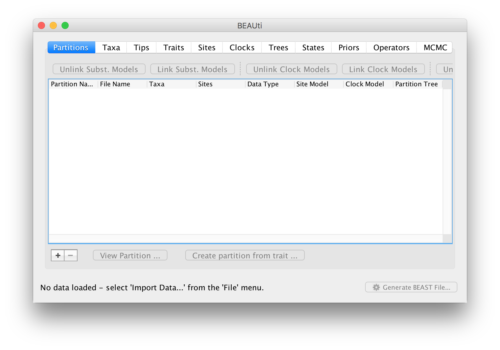
The first thing you need to do is to load some data, in this case a small nucleotide alignment.
To load a NEXUS format alignment, simply select the Import Data... option from the File menu. You can also click the + button at the bottom left of the window or just drag-and-drop the file into the main window.
The NEXUS alignment
This file contains an alignment of mitochondrial tRNA sequences from 6 primate species (5 apes and a monkey outgroup). It starts out like this (the lines have been truncated):
#NEXUS

BEGIN DATA;
	DIMENSIONS NTAX=6 NCHAR=768;
	FORMAT MISSING=? GAP=- DATATYPE=DNA;
	MATRIX
	human      AGAAATATGTCTGATAAAAGAGTTACTTTGATAGAGTAAATAATAGGAGC...
	chimp      AGAAATATGTCTGATAAAAGAATTACTTTGATAGAGTAAATAATAGGAGT...
	bonobo     AGAAATATGTCTGATAAAAGAATTACTTTGATAGAGTAAATAATAGGAGT...
	gorilla    AGAAATATGTCTGATAAAAGAGTTACTTTGATAGAGTAAATAATAGAGGT...
	orangutan  AGAAATATGTCTGACAAAAGAGTTACTTTGATAGAGTAAAAAATAGAGGT...
	siamang    AGAAATACGTCTGACGAAAGAGTTACTTTGATAGAGTAAATAACAGGGGT...
	;
END;
BEAST can also import FASTA files (as long as the sequences have been aligned) or BEAST XML files (in which case the data will imported but the models and settings will not).
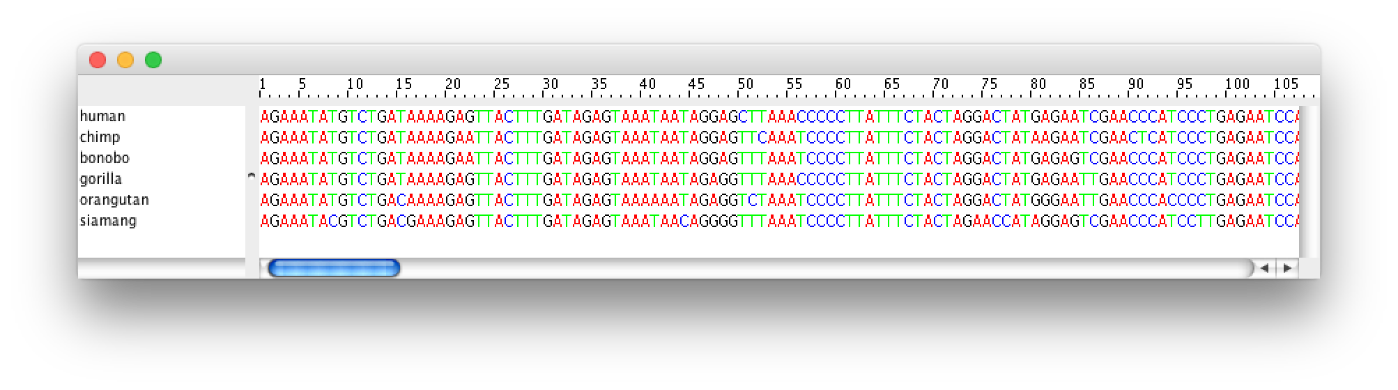
Once loaded, the alignment will be displayed in the main window in a table:
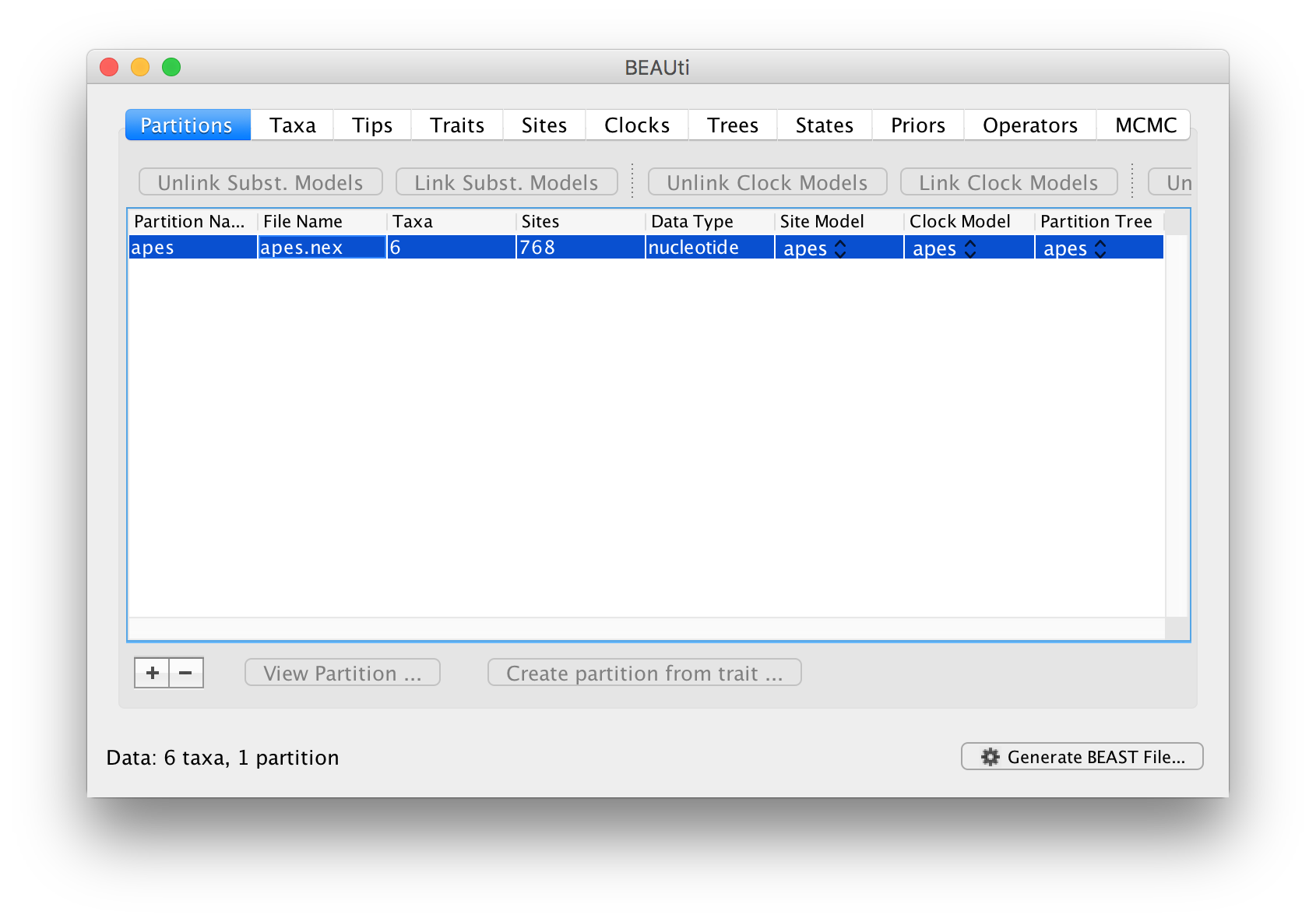
If you want to look at the actual alignment, double click on the row in the table.
Along the top of the main window is a strip of ‘tabs’:

Each of these has settings and options and in general you should work from left to right (although not all the tabs will be relevant to all analyses). After the Partitions tab where you imported data, skip the Taxa tab for now and move straight on to the Tips tab.
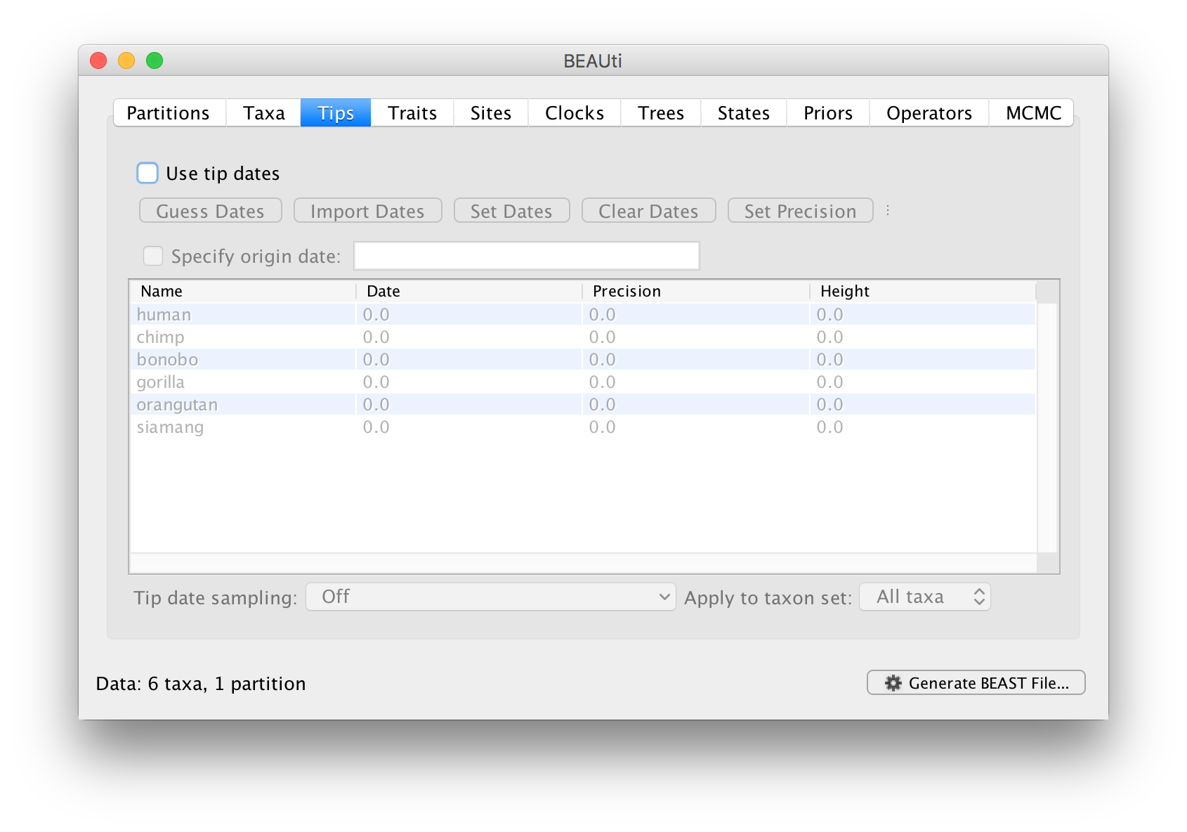
Setting the dates of the taxa
In the Tips options you will see a table with all of the taxa that were in the alignment. This panel allows you go give the taxa dates. Taxon dates (or ‘tip dates’) are only important in certain cases, for example, when they sampled from fast evolving viruses or sub-fossil ancient DNA material. In the case of the apes we are analysing the tree represents millions of years of evolution so the dates of the tips can be assumed to be zero. This is the default — the taxa all have a date of zero and the Use tip dates box is not selected.
Skip the Traits tab and move on to the Sites tab.
Setting the evolutionary model
In the Sites tab you can set the model of molecular evolution for the sequence data you have loaded. Exactly which options appear depend on whether the data are nucleotides or amino acids (or other forms of data). The settings that will appear after loading the apes.nex data set will be as follows:
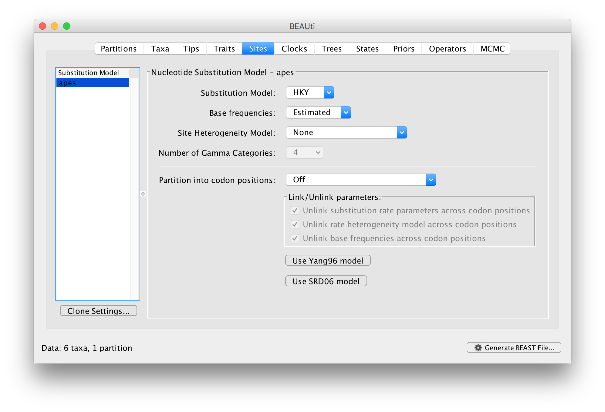
This tutorial assumes you are familiar with the evolutionary models available, however there are a couple of points to note:
The default is a simple HKY (Hasegawa, Kishino & Yano (1985) J Mol Evol 22: 160-174) model of nucleotide evolution. We are going to use this model.
Setting the molecular clock model
In the next tab Clock we set the model of molecular clock we will use. Unlike many other phylogenetic software BEAST exclusively uses molecular clock models so that trees have a timescale (an inferred root and direction in time). The simplest model is the default ‘Strict clock’. This assumes that all branches on the tree have the same rate of evolution. The other molecular clock models relax this assumptions in various ways which later tutorials will discuss.
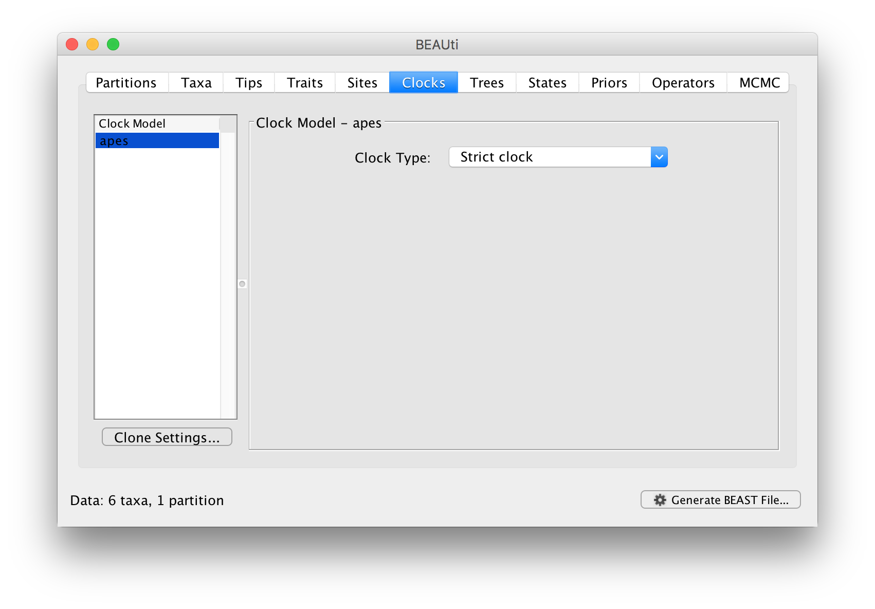
For this analysis leave the Clock Type as Strict clock and move on to the Trees tab.
Setting the tree prior model
In this panel you can set the model that provides a prior on the tree and some choices about the starting tree in the MCMC run.
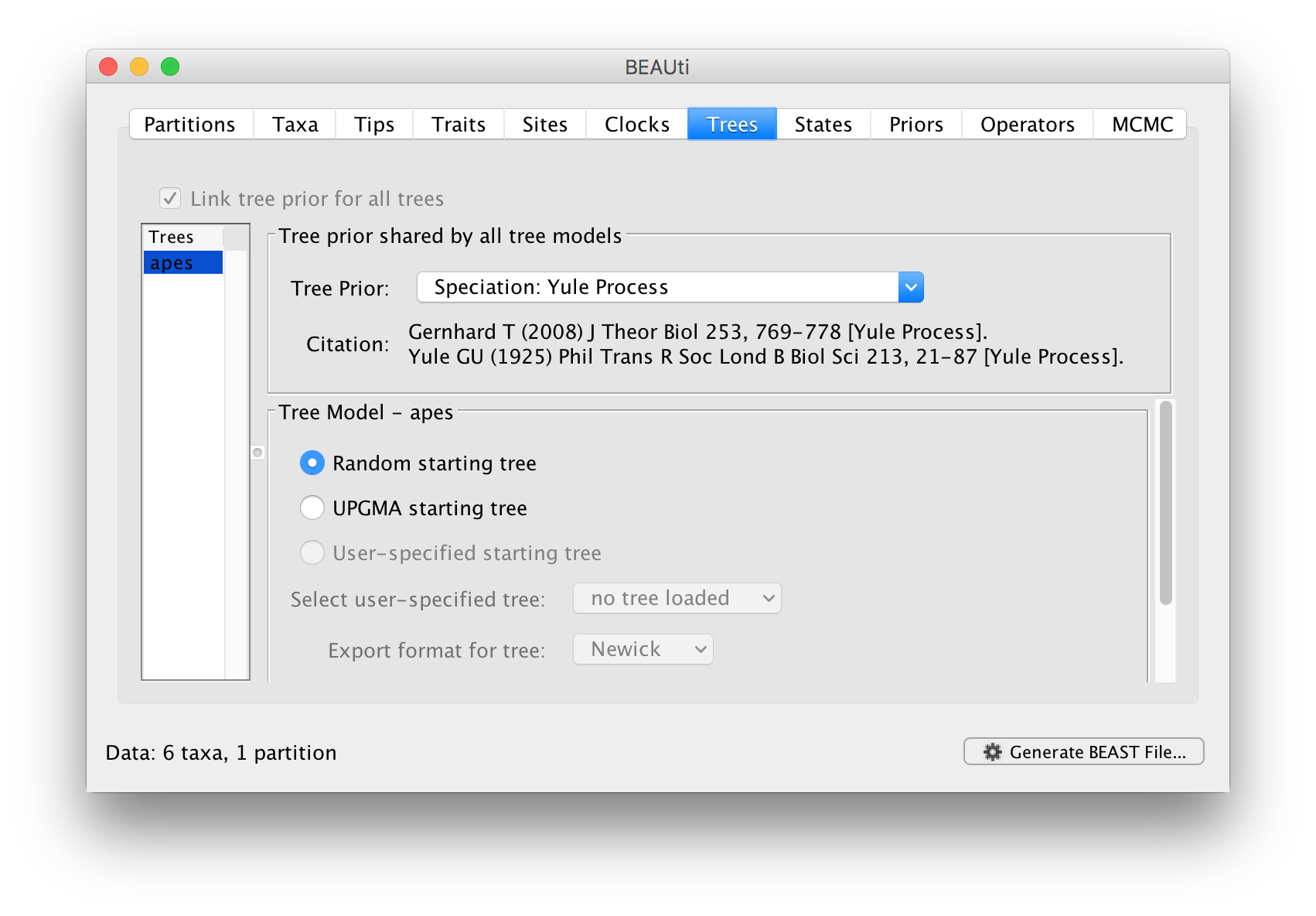
The Tree Prior option has many choices divided generally into ‘Coalescent’ models which are generally suited to populations and ‘Speciation’ models which, as the name suggests are intended for species level data. As we have sequence data from a handful of species, we will select the Speciation: Yule process model. The Yule process Yule (1925) Phil Trans Royal Soc B 213: 402-420 is the simplest model of speciation where each lineage is assumed to have speciated at a fixed rate. The model has a single parameter, the ‘birth rate’ of new species.
The bottom half of this panel allows you to choose how BEAST selects a starting tree. In most situations it is better to leave this as Random starting tree. This generates a random tree to start the BEAST run with.
Select the Yule process and move to the next Priors tab.
Priors
The next tab allows priors to be specified for each parameter in the model:
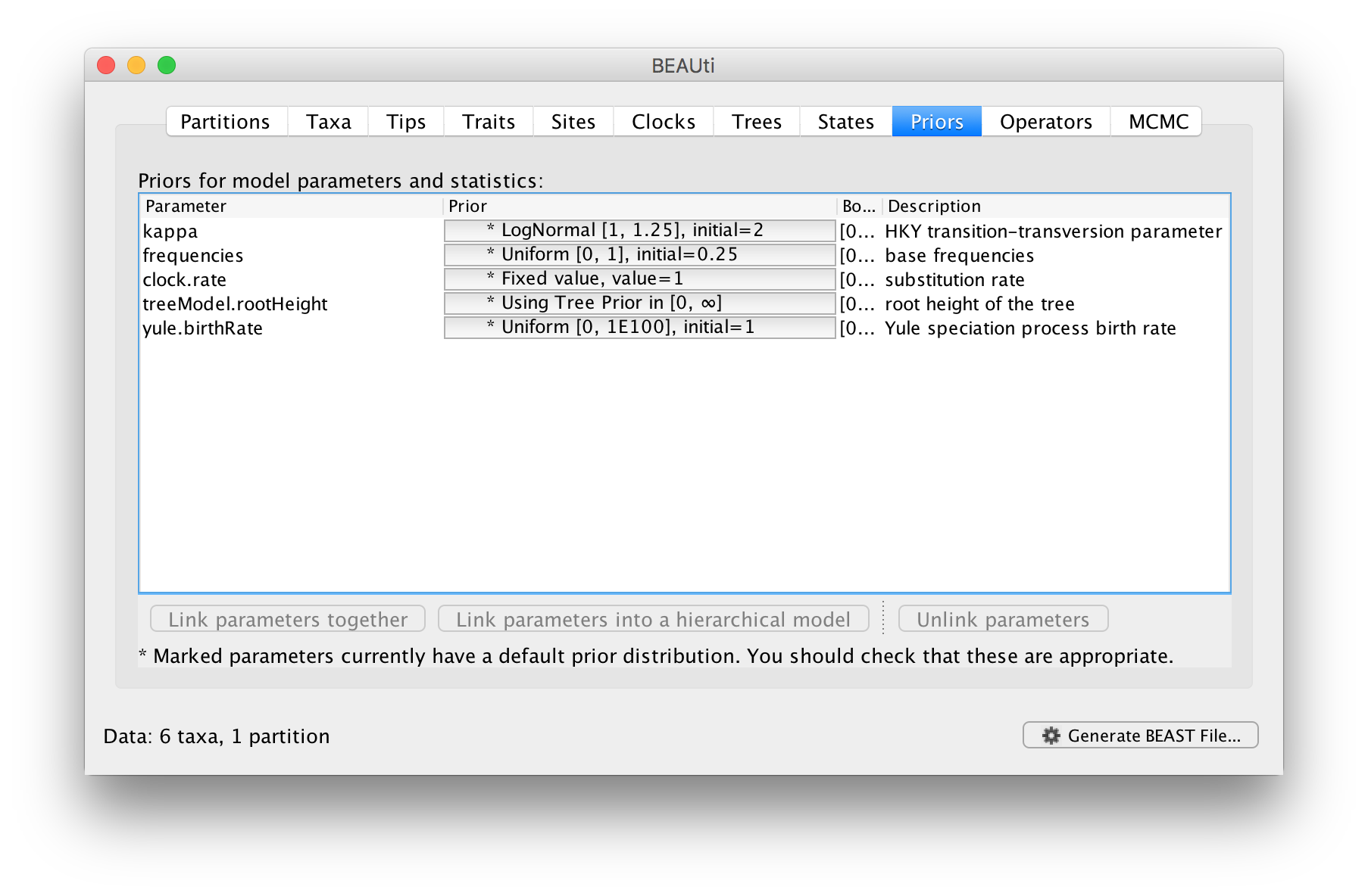
Selecting priors is one of the most challenging aspects of Bayesian analysis. In BEAST we have tried to pick some reasonably appropriate and robust priors as defaults for most parameters. In this tutorial, the default options will be used.
MCMC operators
The next stage is to look at the operators for the MCMC. To do this select the Operators tab at the top of the main window. For the ape.nex dataset, with the model set up as shown in the screen shot above, you will see the following table:
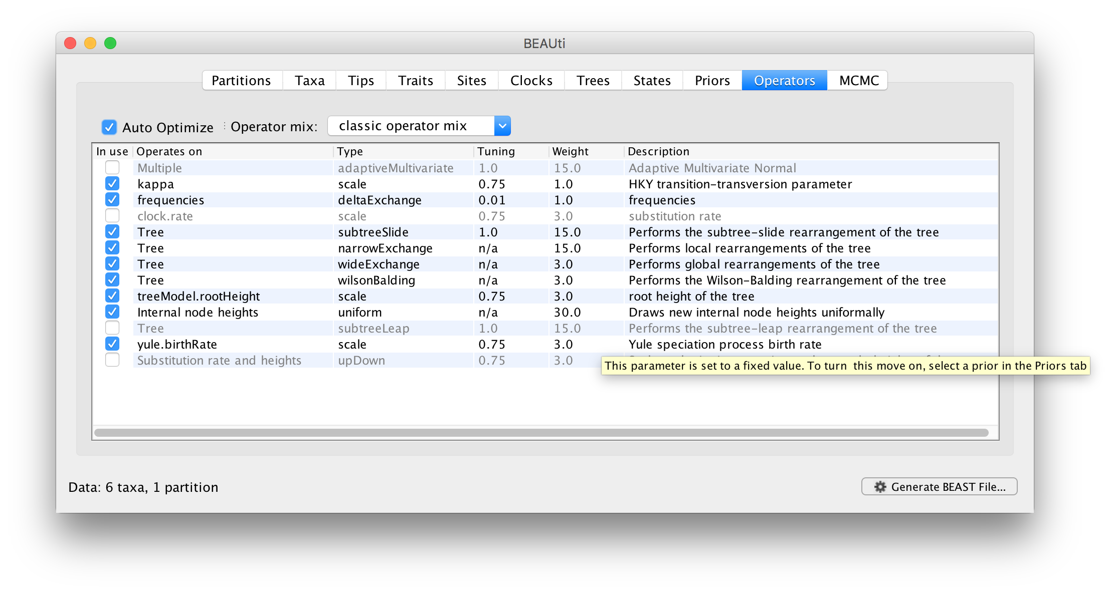
Each parameter in the model has one or more “operators”. The operators specify how the parameter changes as the MCMC runs. This table lists the parameters, their operators and the tuning settings for these operators. In the first column are the parameter names. These will be called things like kappa which means the HKY model’s kappa parameter (the transition-transversion bias). The next column has the type of operators that are acting on each parameter. For example, the scale operator scales the parameter up or down by a proportion, the random walk operator adds or subtracts an amount to the parameter and the uniform operator simply picks a new value uniformally within a range. Some parameters relate to the tree or to the heights of the nodes of the tree and these have special operators.
The next column, labelled Tuning, gives a tuning setting to the operator. Some operators don’t have any tuning settings so have n/a under this column. Changing the tuning setting will set how large a move that operator will make which will affect how often that change is accepted by the MCMC which will affect the efficency of the analysis. At the top of the window is an option called Auto Optimize which, when selected, will automatically adjust the tuning setting as the MCMC runs to try to achieve maximum efficiency.
The next column, labelled Weight, specifies how often each operator is applied relative to each other. Some parameters have very little interaction with the rest of the model and as a result tend to be estimated very efficiently - an example is the kappa parameter - these parameters can have their operators down-weighted so that they are not changed as often.
Once again leave the settings at their defaults and move on to the next tab.
Setting the MCMC options
The last tab, MCMC, provides settings to control the actual running of BEAST:
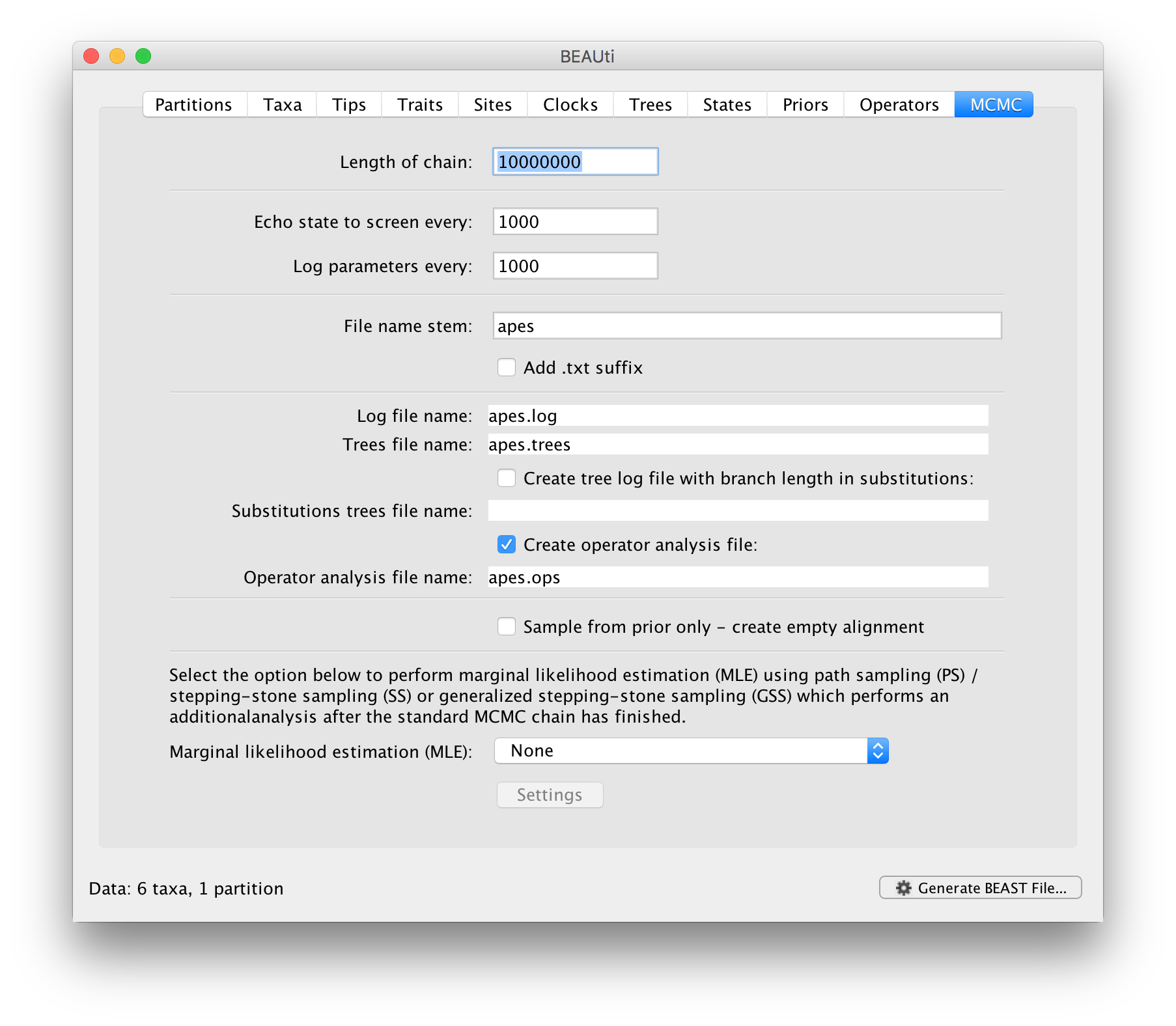
Firstly we have the Length of chain. This is the number of steps the MCMC will make in the chain before finishing. How long this should be depends on the size of the dataset, the complexity of the model and the quality of answer required. The default value of 10,000,000 is entirely arbitrary and should be adjusted according to the size of your dataset. In order examine whether a particular chain length is adequate, the resulting log file can be analysed using Tracer. The aim of setting the chain length is to achieve a reasonable Effective Sample Size (ESS). Ways of doing this are discussed in another tutorial.
The next options specify how often the current parameter values should be displayed on the screen and recorded in the log file. The screen output is simply for monitoring the programs progress so can be set to any value (although if set too small, the sheer quantity of information being displayed on the screen may actually slow the program down). For the log file, the value should be set relative to the total length of the chain. Sampling too often will result in very large files with little extra benefit in terms of the precision of the analysis. Sample too infrequently and the log file will not contain much information about the distributions of the parameters. You probably want to aim to store about 10,000 samples so this should be set to the chain length / 10,000.
For this dataset (which is very small) let’s initially setting the chain length to 1,000,000 as this will run very quickly on most modern computers. Set the sampling frequency to 100, accordingly.
Echo state to screen option to 10000 resulting in only 100 updates to the screen as the analysis runs.The final two options give the file names of the log files for the parameters and the trees. These will be set to a default based on the name of the imported NEXUS file but feel free to change these. The rest of the options can be ignored for the purposes of this tutorial.
.txt to the log and the trees file — Windows will hide the .txt but still show you the .log and .trees extensions so you can distinguish the files.Saving and Loading BEAUti files
If you select the Save option from the File menu this will save a document in BEAUti’s own format. Note that is not in the format that BEAST understands — it can only be reopened by BEAUti. The idea is that the settings and data in BEAUti can be saved and loaded at a later time. We suggest you save BEAUti files with the extension ‘.beauti’.
Generating the BEAST XML file
We are now ready to create the BEAST XML file. Select Generate XML... from the File menu (or the button at the bottom of the windo) and save the file with an appropriate name — it will offer the name you gave it in the MCMC panel and we usually end the filename with ‘.xml’ (although see the note, above, about extensions on Windows machines – you may want to give the file the extension ‘.xml.txt’).
We are now ready to run the file through BEAST.
Running BEAST
The following dialog box will appear:
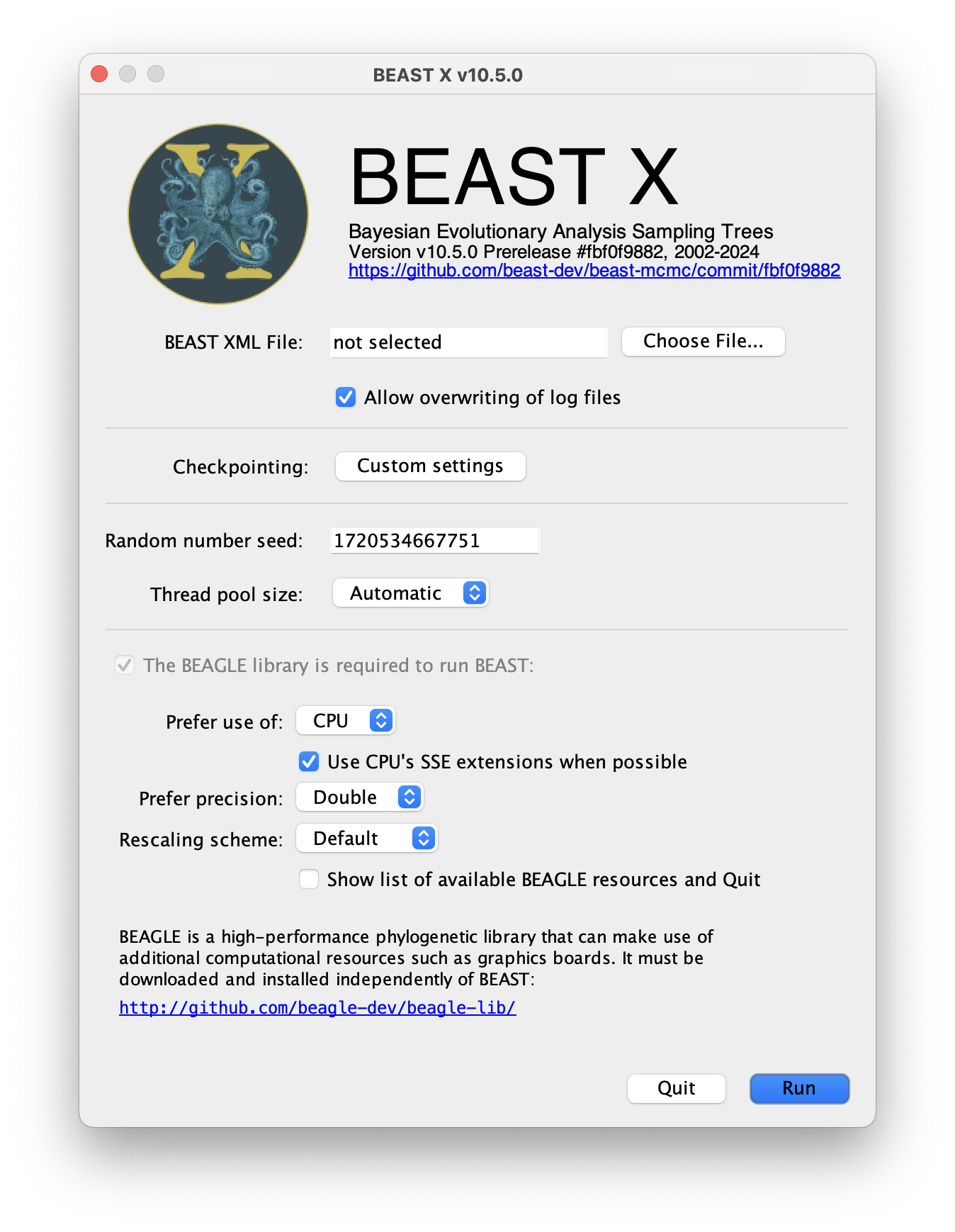
All you need to do is to click the Choose File... button, select the XML file you created in BEAUti, above, and press Run. For information about the other options see the page on the BEAST program.
When you press Run BEAST will load the XML file, setup the analysis and then run it with no further interaction. In the output window you will see lots of information appearing. It starts by printing the title and credits:
                   BEAST X v10.x, 2002-2102
       Bayesian Evolutionary Analysis Sampling Trees
                 Designed and developed by
   Alexei J. Drummond, Andrew Rambaut and Marc A. Suchard

               Department of Computer Science
                   University of Auckland
                  alexei@cs.auckland.ac.nz

             Institute of Evolutionary Biology
                  University of Edinburgh
                     a.rambaut@ed.ac.uk

              David Geffen School of Medicine
           University of California, Los Angeles
                     msuchard@ucla.edu

                Downloads, Help & Resources:
                 	http://beast.community

Source code distributed under the GNU Lesser General Public License:
          	http://github.com/beast-dev/beast-mcmc
Then it gives some details about the data it loaded and the models you have specified. You should see that it has repeated all of the choices you made in BEAUti.
Random number seed: 1500828054875

Parsing XML file: apes.xml
  File encoding: UTF8
Looking for plugins in /Users/rambaut/Projects/BEAST/plugins

Read alignment: alignment
  Sequences = 6
      Sites = 768
   Datatype = nucleotide
Site patterns 'patterns' created from positions 1-768 of alignment 'alignment'
  unique pattern count = 69

Using Yule prior on tree

Creating the tree model, 'treeModel'
  initial tree topology = ((((bonobo,human),orangutan),gorilla),(chimp,siamang))
  tree height = 102.55912280908296

Using strict molecular clock model.

Creating state frequencies model 'frequencies': Initial frequencies = {0.25, 0.25, 0.25, 0.25}

Creating HKY substitution model. Initial kappa = 2.0

Creating site rate model:
  with initial relative rate = 1.0

Using Multi-Partition Data Likelihood Delegate with BEAGLE 3 extensions
  Using BEAGLE resource 0: CPU
    with instance flags:  PRECISION_DOUBLE COMPUTATION_SYNCH EIGEN_REAL SCALING_MANUAL SCALERS_RAW VECTOR_SSE THREADING_NONE PROCESSOR_CPU FRAMEWORK_CPU
  Ignoring ambiguities in tree likelihood.
  With 1 partitions comprising 69 unique site patterns
  Using rescaling scheme : dynamic (rescaling every 100 evaluations, delay rescaling until first overflow)

Using TreeDataLikelihood
Optimization Schedule: default

Likelihood computation is using an auto sizing thread pool.

Creating the MCMC chain:
  chainLength=1000000
  autoOptimize=true
  autoOptimize delayed for 10000 steps
Next it prints out a block of citations for BEAST and for the individual models and components selected. This is intended to help you write up the analysis, specifying and citing the models used:
Citations for this analysis:

FRAMEWORK
BEAST primary citation:
	Drummond AJ, Suchard MA, Xie Dong, Rambaut A (2012) Bayesian phylogenetics with BEAUti and the BEAST 1.7. Mol Biol Evol. 29, 1969-1973. DOI:10.1093/molbev/mss075

TREE DENSITY MODELS
Gernhard 2008 Birth Death Tree Model:
	Gernhard T (2008) The conditioned reconstructed process. Journal of Theoretical Biology. 253, 769-778. DOI:10.1016/j.jtbi.2008.04.005

SUBSTITUTION MODELS
HKY nucleotide substitution model:
	Hasegawa M, Kishino H, Yano T (1985) Dating the human-ape splitting by a molecular clock of mitochondrial DNA. J. Mol. Evol.. 22, 160-174
Finally BEAST starts to run. It prints up various pieces of information that is useful for keeping track of what is happening. The first column is the ‘state’ number — in this case it is incrementing by 1000 so between each of these lines it has made 1000 operations. The screen log shows only a few of the metrics and parameters but it is also recording a log file to disk with all of the results in it (along with a ‘.trees’ file containing the sampled trees for these states).
After a few thousand states it will start to report the number of hours per million states (or if it is running very fast, per billions states). This is useful to allow you to predict how long the run is going to take and whether you have time to go and get a cup of coffee, or lunch, or a two week vacation in the Caribbean.
# BEAST v1.X
# Generated Sun Jul 23 17:42:37 BST 2017 [seed=1500828054875]
state	Posterior   	Prior       	Likelihood  	rootAge
0	-6812.7534  	-481.7973   	-6330.9561  	102.559     	-
10000	-2910.2955  	-246.4611   	-2663.8344  	13.7383     	-
20000	-2082.7664  	-234.0125   	-1848.7539  	0.12112     	-
30000	-2049.3031  	-230.0213   	-1819.2818  	5.84813E-2  	-
40000	-2043.1005  	-226.3604   	-1816.7401  	6.21508E-2  	-
50000	-2042.1593  	-226.1915   	-1815.9678  	5.79924E-2  	-
.
.
.
After waiting the expected amount of time, BEAST will finish.
950000	-2044.0265  	-227.1010   	-1816.9255  	5.98269E-2  	11.27 hours/billion states
960000	-2041.6364  	-225.0546   	-1816.5818  	5.58888E-2  	11.27 hours/billion states
970000	-2046.3378  	-227.5622   	-1818.7756  	5.96169E-2  	11.27 hours/billion states
980000	-2039.9261  	-226.1422   	-1813.7839  	5.96151E-2  	11.27 hours/billion states
990000	-2047.3466  	-227.6691   	-1819.6775  	6.41662E-2  	11.27 hours/billion states
1000000	-2040.3296  	-225.5095   	-1814.8201  	5.74639E-2  	11.27 hours/billion states

Operator analysis
Operator                                          Tuning   Count      Time     Time/Op  Pr(accept)
scale(kappa)                                      0.239   13605      621      0.05     0.2453
frequencies                                       0.105   13530      722      0.05     0.2398
subtreeSlide(treeModel)                           0.025   202546     5651     0.03     0.2313
Narrow Exchange(treeModel)                                203114     7020     0.03     0.0547
Wide Exchange(treeModel)                                  40112      623      0.02     0.0099
wilsonBalding(treeModel)                                  40753      848      0.02     0.0053
scale(treeModel.rootHeight)                       0.148   40635      1192     0.03     0.2406
uniform(nodeHeights(treeModel))                           404956     13096    0.03     0.385
scale(yule.birthRate)                             0.126   40749      305      0.01     0.2392

41.987 seconds
The table at the end lists each of the operators, how many times each was used, how much time they took and some other details. This information can be useful for optimising the performance of runs but generally it can be ignored.
This took 40 seconds to run on a low-performance MacBook. Clearly we would be able to run it for much longer whilst getting a coffee but with such a small data set we may not need to. We will find out when we start to look at the output files from BEAST.