Phylogeographic Diffusion in Continuous Space - WNV example

Introduction

The first step will be to convert an alignment file in fasta format into a BEAST XML input file. This is done using the program BEAUti (this stands for Bayesian Evolutionary Analysis Utility). This is a user-friendly program for setting the evolutionary model and options for the MCMC analysis. The second step is to actually run BEAST using the input file that contains the data, model and settings. The final step is to explore the output of BEAST in order to diagnose problems and to summarize the results.

To undertake this tutorial, you will need to download three software packages in a format that is compatible with your computer system (all three are available for Mac OS X, Windows and Linux/UNIX operating systems):

BEAST - this package contains the BEAST program, BEAUti and a couple of utility programs. At the time of writing, the current version is v10.5.0-beta5. BEAST releases are available for download from https://github.com/beast-dev/beast-mcmc/releases.

BEAGLE - this is a high-performance library that can perform the core calculations at the heart of most Bayesian and Maximum Likelihood phylogenetics packages. It can make use of highly-parallel processors such as those in graphics cards (GPUs) found in many PCs. Binary installers and installation instructions can be found at https://github.com/beagle-dev/beagle-lib.

Tracer - this program is used to explore the output of BEAST (and other Bayesian MCMC programs). It graphically and quantitively summarizes the empirical distributions of continuous parameters and provides diagnostic information. At the time of writing, the current version is v1.7.2. It is available for download from https://github.com/beast-dev/tracer/.

FigTree - this is an application for displaying and printing molecular phylogenies, in particular those obtained using BEAST. At the time of writing, the current version is v1.4.4. It is available for download from https://github.com/rambaut/figtree/.

SpreaD3 - this is an application for the visualization of phylogeographic analyses performed with BEAST. At the time of writing, the current version is v0.9.7.1. It is available for download from https://rega.kuleuven.be/cev/ecv/software/SpreaD3.

Running BEAUti

The program BEAUti is a user-friendly program for setting the model parameters for BEAST. Run BEAUti by double clicking on its icon.

Loading the sequence data file

To load the alignment, simply select the Import Data... option from the File menu:

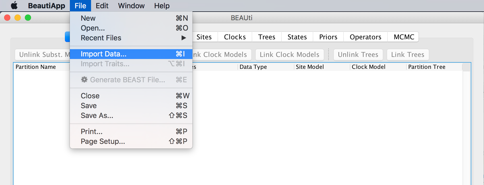
and browse to the WNV.fas file to load it.

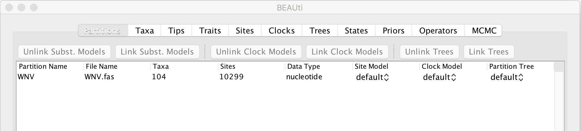
Select the WNV.fas file. This file contains an alignment of 104 WNV genomes 11029 nucleotides in length. Once loaded, the sequence data will be listed under Partitions as shown in the figure:

Specifying the sampling date information

By default all the taxa are assumed to have a date of zero (i.e. the sequences are assumed to be sampled at the same time). In this case, the WNV sequences have been sampled at various years going back to 1999. To set these dates switch to the Tips panel using the tabs at the top of the window.

Select the box labelled Use tip dates. The actual sampling time in years is encoded in the name of each taxon and we could simply edit the value in the ‘Date’ column of the table to reflect these. However, if the taxa names contain the calibration information, then a convenient way to specify the dates of the sequences in BEAUti is to use the Parse Dates button at the top left of the Data panel. Clicking this will make a dialog box appear:

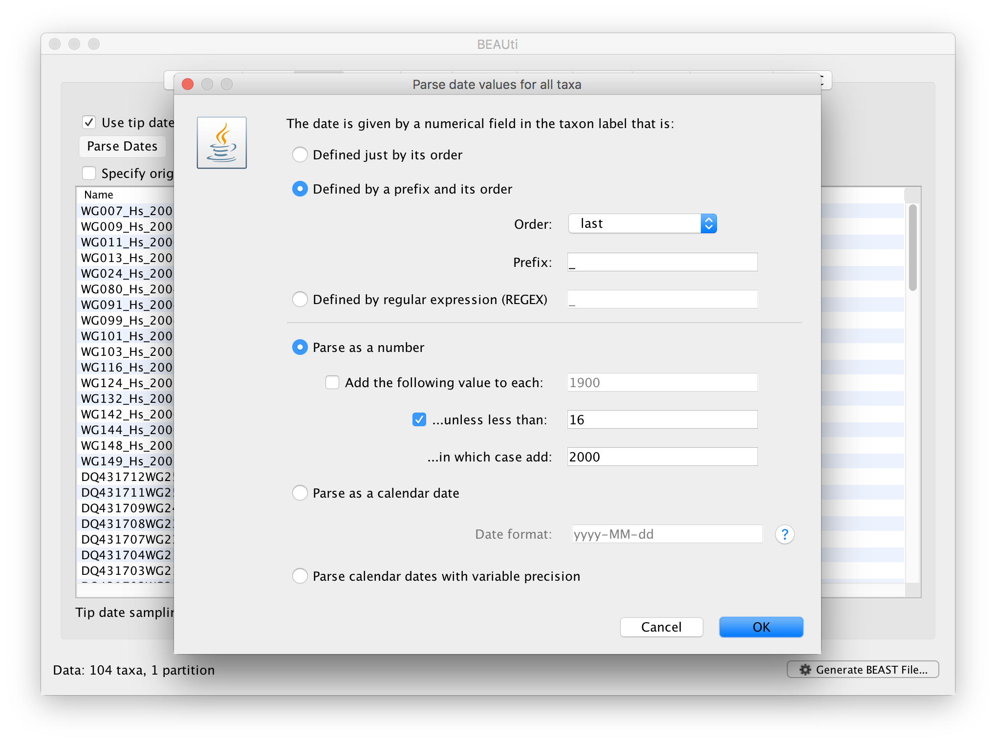
This operation attempts to guess what the dates are from information contained within the taxon names. It works by trying to find a numerical field within each name. If the taxon names contain more than one numerical field then you can specify how to find the one that corresponds to the date of sampling. You can (1) specify the order that the date field comes (e.g., first, last or various positions in between) or (2) specify a prefix (some characters that come immediately before the date field in each name) and the order of the field, or (3) define a regular expression (REGEX).

When parsing a number, you can ask BEAUti to add a fixed value to each guessed date. For example, the value 1900 can be added to turn the dates from 2 digit years to 4 digit. Any dates in the taxon names given as 00 would thus become 1900. However, if these 00 or 01, etc. represent sequences sampled in 2000, 2001, etc., 2000 needs to be added to those. This can be achieved by selecting the unless less than: .. and ..in which case add:.. options adding for example 2000 to any date less than 10. These operations are not necessary in our case since the dates are fully specified at the end of the sequence names. There is also an option to parse calendar dates and one for calendar dates with various precisions. For the WNV sequences you can keep the default Defined just by its order, select last from the drop-down menu for the order, set the Prefix to an underscore and press OK. The dates will appear in the appropriate column of the main window.

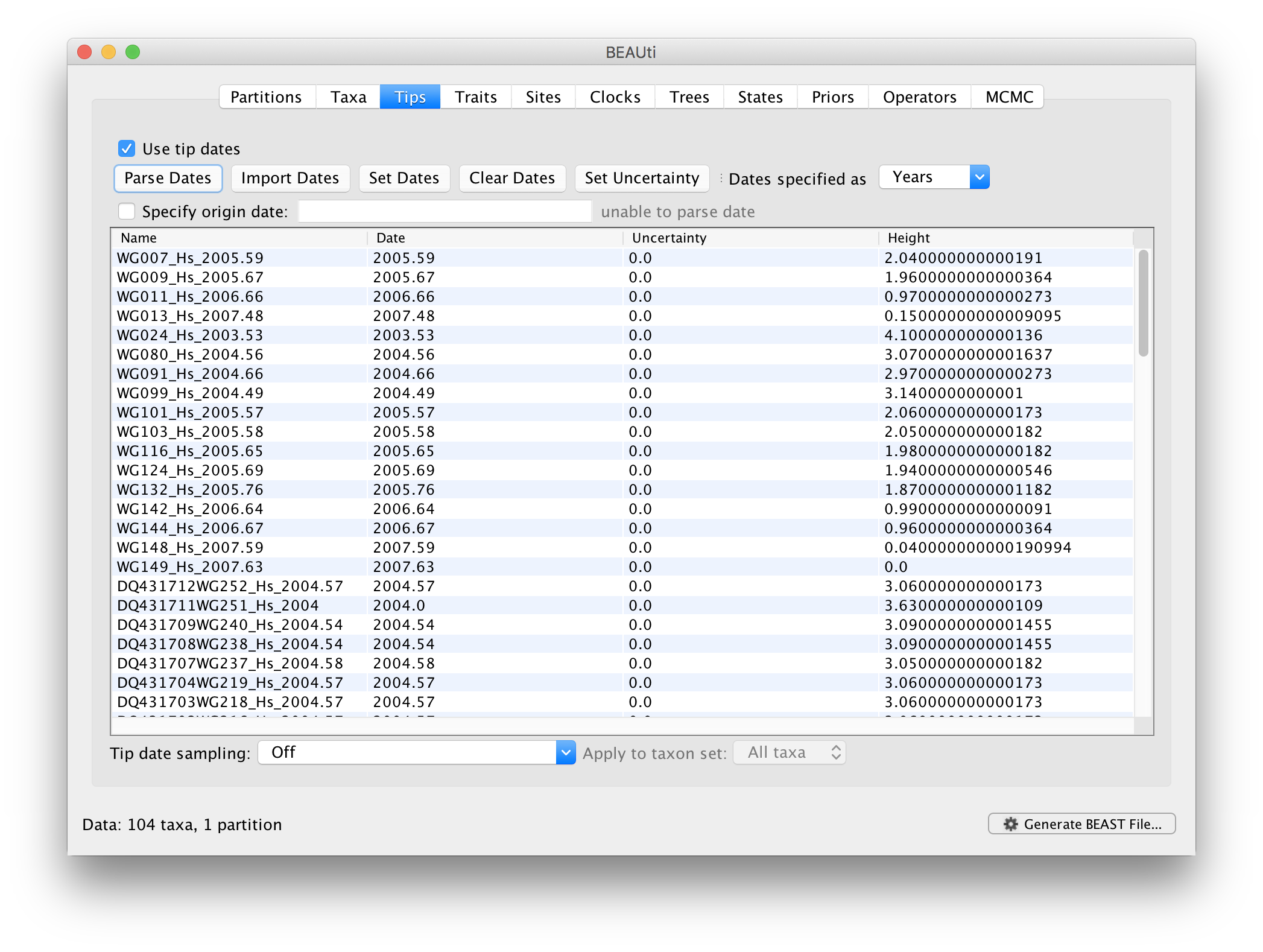
You can now check these and edit them manually as required. At the top of the window you can set the units that the dates are given in (years, months, days) and whether they are specified relative to a point in the past (as is the case for years such as 2005) or backwards in time from the present (as in the case of radiocarbon ages).

The Height column lists the ages of the tips relative to time 0 (in our case 2007.63). The Uncertainty column allows specifying with what precision the sampling time is know. This is useful in our case because some sampling dates are known to the exact day, while others are only known up to the year of sampling (those without decimal in the taxa name or with the .0 decimal in the Date column), and BEAST allows to integrate over the uncertainty of the latter. To make use of the ability to adequately accommodate the uncertainty of our sampling dates, select all the taxa (holding down the cmd key) with sampling dates only known up to the year in the Tips window and click on Set Uncertainty.

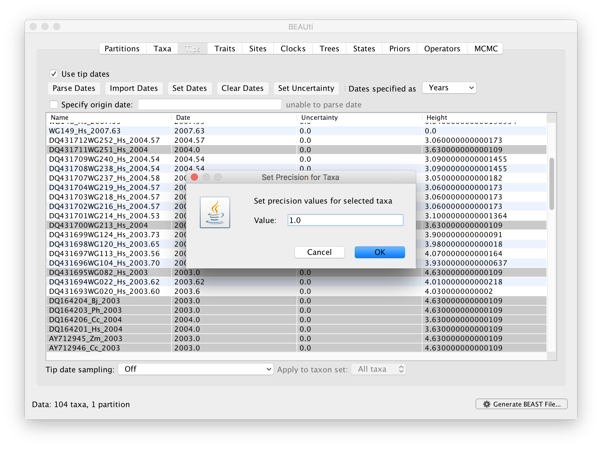
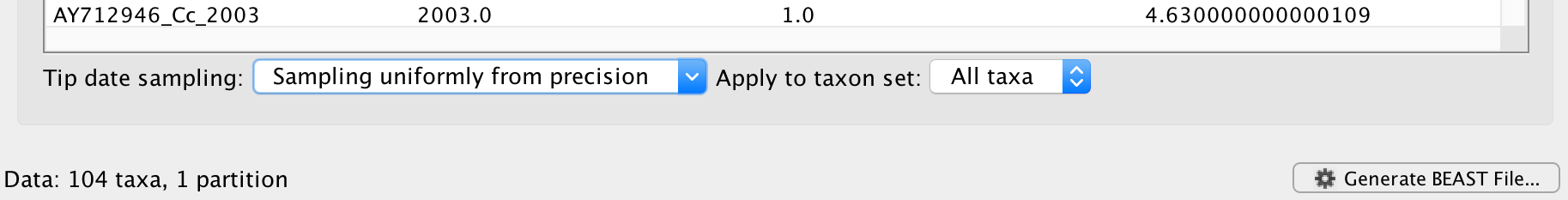
Enter ‘1.0’ as the precision value for 1 year. This will instruct BEAST to add a half year to those sampling dates and construct a uniform window of 1 year around this new value. To estimate the respective sampling dates within the constraint of this window in the MCMC analysis, select sampling uniformly from precision at the bottom left of the Tips panel and keep the Apply to taxon set: All taxa default.

Specifying the trait information

The next thing to do is to click on the Traits tab at the top of the main window. A trait can be any characteristic that is inherent to the specific taxon, for example, geographical location or host species. This step will assign a latitude and longitude as bivariate geographical location to each taxa based on the trait specification for each sequence.

To associate the sequences with the traits, we need to import a new trait under the Traits tab (click Import Traits...). This will open a new window that allows importing a file with the traits. Browse to and Open the WNV_lat_long.txt tab-delimited file, with the following content:

traits	lat	long
WG007_Hs_2005.59	31.82	-106.56
WG009_Hs_2005.67	32.28	-106.74
WG011_Hs_2006.66	31.78	-106.50
WG013_Hs_2007.48	31.84	-106.53
WG024_Hs_2003.53	33.81	-117.83
WG080_Hs_2004.56	34.22	-118.44
WG091_Hs_2004.66	34.14	-117.15
WG099_Hs_2004.49	34.04	-117.02
WG101_Hs_2005.57	33.95	-117.73
WG103_Hs_2005.58	33.85	-118.15
WG116_Hs_2005.65	33.84	-118.08
WG124_Hs_2005.69	32.31	-111.21
	...
DQ080059\_Pn\_2003	38.58	-121.49

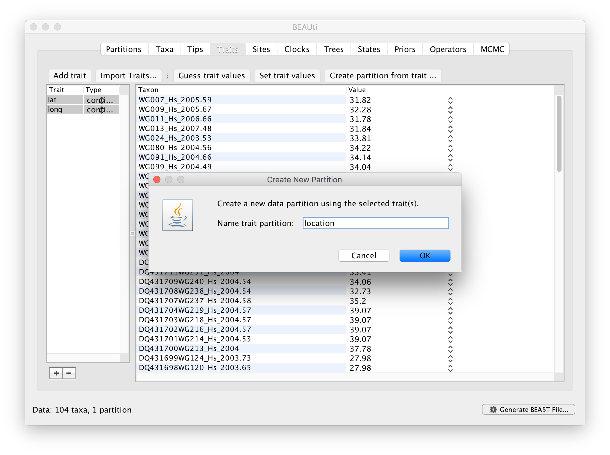
After clicking OK, select both the ‘lat’ and ‘long’ trait in the left window and click on create partition from trait... In the window that pops up, enter a name for this partitions, e.g. ‘location’:

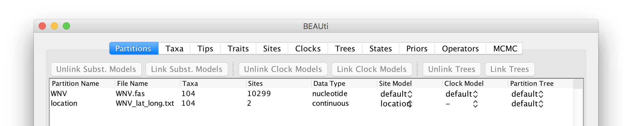
This new ‘location’ partition with 2 ‘Sites’ and with a continuous ‘Data Type’ will be shown under the Partitions tab:

Setting the sequence and trait evolutionary models

The next thing to do is to click on the Sites tab at the top of the main window. This will reveal the evolutionary model settings for BEAST. Exactly which options appear depend on whether the data are nucleotides, amino acids or traits.

This tutorial assumes that you are familiar with the available evolutionary models, however there are a couple of points to note about selecting a model in BEAUti:

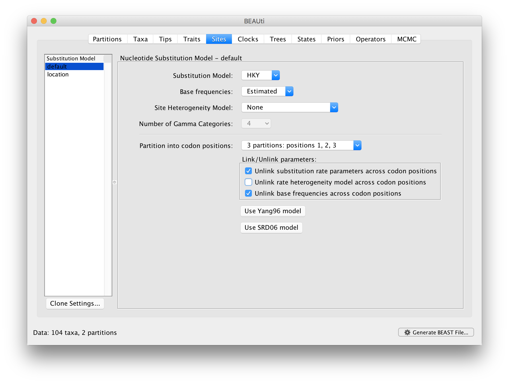
Selecting the Partition into codon positions option assumes that the data are aligned as codons. This option will then estimate a separate rate of substitution for each codon position, or for 1+2 versus 3, depending on the setting.

Selecting the Unlink substitution model across codon positions will specify that BEAST should estimate a separate transition-transversion ratio or general time reversible rate matrix for each codon position.

Selecting the Unlink rate heterogeneity model across codon positions will specify that BEAST should estimate a set of rate heterogeneity parameters (gamma shape parameter and/or proportion of invariant sites) for each codon position.

For the nucleotide substitution model in this tutorial, keep the default HKY substitution model, keep the base frequencies to be ‘Estimated’, the ‘Site Rate Heterogeneity’ to ‘None’, and partition the data into 3 partitions for the coding positions (3 partitions: positions 1,2,3). Because of the renaissance counting procedure that we will apply to obtain site-specific dN/dS estimates, we cannot model rate heterogeneity within each codon position partition, so we will assume that we capture most among site rate heterogeneity by modeling relative rates among the coding position partitions.

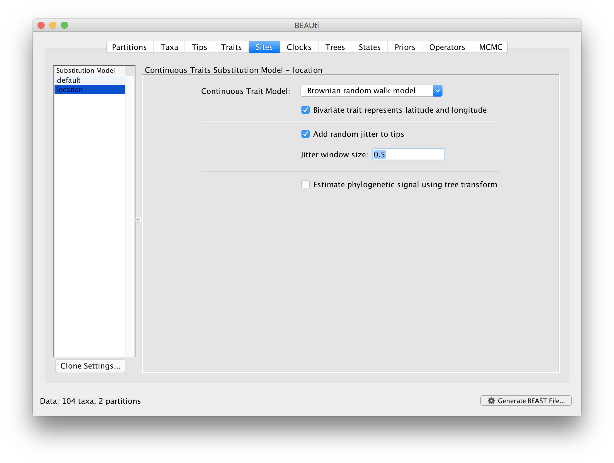
Next, click on ‘location’ in the Substitution model window and keep the Homogenous Brownian model, and select Bivariate trait represents latitude and longitude. This option generates diffusion statistics that are specific for bivariate spatial traits (with latitude and longitude in that order). Also select the add random jitter to tips, which adds noise drawn uniformly at random from a particular jitter window size to duplicated (location) traits. Set the jitter window size to 0.5. The noise avoids a poor performance of Brownian diffusion models when not all sequences are associated with unique locations.

Setting the ‘molecular clock’ model

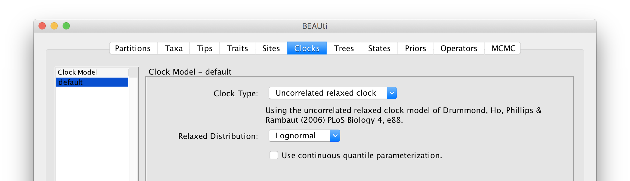
The ‘Molecular Clock Model’ options in the Clocks panel allows us to choose between a strict and a relaxed (uncorrelated lognormal or uncorrelated exponential) clock. We will perform our run using the Lognormal relaxed molecular clock (Uncorrelated) model:

Now move on to the Trees panel.

Setting the tree prior

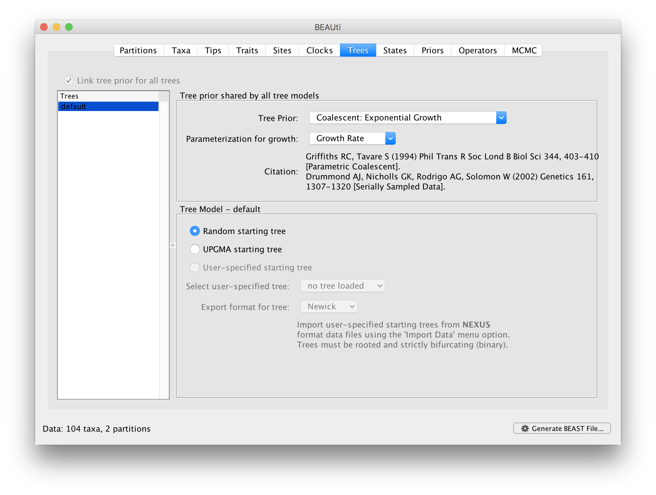
This panel contains settings about the tree. Firstly the starting tree is specified to be ‘randomly generated’. The other main setting here is to specify the ‘Tree prior’ which describes how the population size is expected to change over time according to a coalescent model. The default tree prior is set to a constant size coalescent prior. We will select an exponential growth coalescent model as demographic tree prior (Coalescent: Exponential Growth) with standard parametrisation, which is intuitively appealing for viral outbreaks.

The ancestral states settings

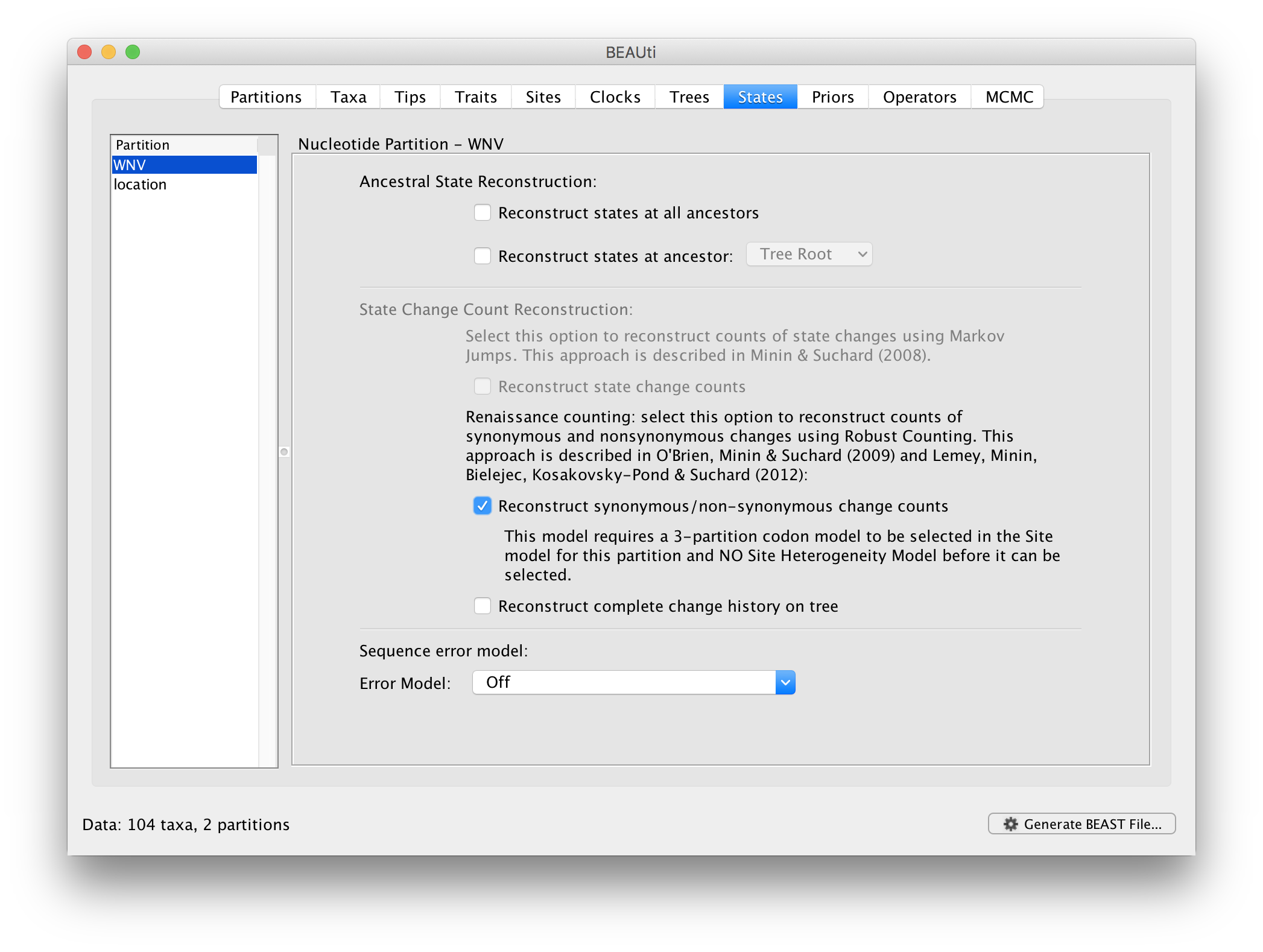
In the States panel, we can turn on the Renaissance counting procedure by selection Reconstruct synonymous/non-synonymous change counts:

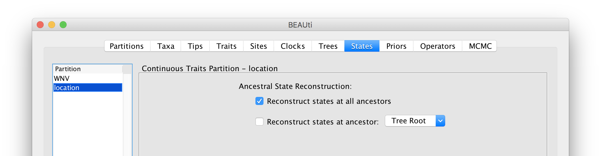
For the ‘location’ partition, check that the option to Reconstruct states at all ancestors is selected (by default):

Setting up the priors

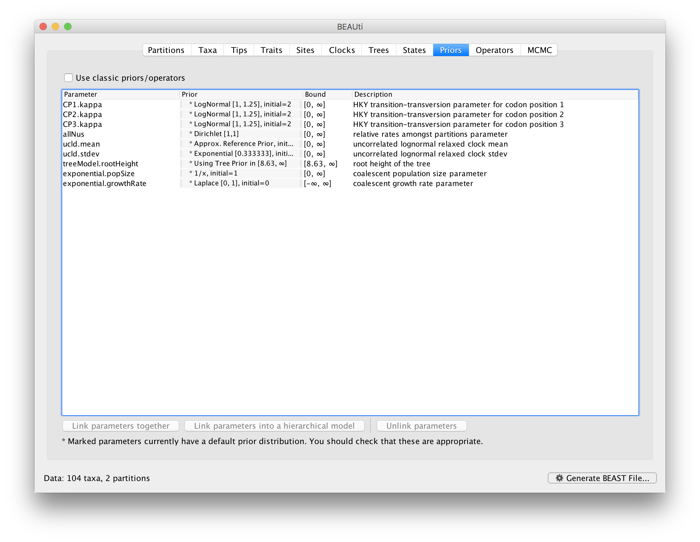
Review the prior settings under the Priors tab. This panel has a table showing every parameter of the currently selected model and what the prior distribution is for each. <Priors that would not be explicitly specified would appear in red, whereas priors that are improper (and hence lead to an improper posterior and improper marginal likelihoods) appear in yellow (e.g. allMus). Click on the prior for this parameter and a prior selection window will appear. The codon position-specific relative rates (CP1.mu, CP2.mu and CP3.mu), which are constrained to have a mean of 1, still require proper priors. We here specify lognormal distributions with a log(mean) of 0.0 and a log(stdev) of 1.5 for these parameters. Notice that the prior setting turns black after confirming this setting by clicking OK.

We can keep the default priors in this case

Setting up the operators

Each parameter in the model has one or more “operators” (these are variously called moves, proposals or transition kernels by other MCMC software packages such as MrBayes and LAMARC). The operators specify how the parameters change as the MCMC runs. The Operators tab in BEAUti has a table that lists the parameters, their operators and the tuning settings for these operators:

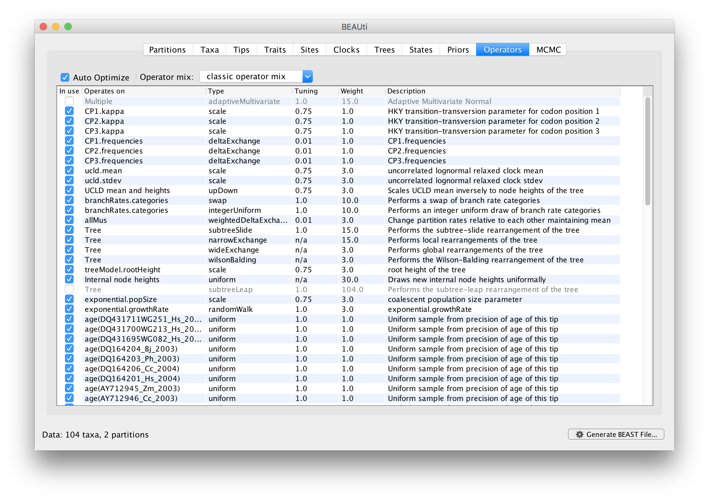
In the first column are the parameter names. These will be called things like kappa which means the HKY model’s kappa parameter (the transition-transversion bias). The next column has the type of operators that are acting on each parameter. For example, the scale operator scales the parameter up or down by a proportion, the random walk operator adds or subtracts an amount to the parameter and the uniform operator simply picks a new value uniformly within a range. Some parameters relate to the tree or to the divergence times of the nodes of the tree and these have special operators. As of BEAST v1.8.4, different options are available w.r.t. exploring tree space. In this tutorial, we will use the ‘classic operator mix’, which consists of of set of tree transition kernels that propose changes to the tree. There is also an option to fix the tree topology as well as a ‘new experimental mix’, which is currently under development with the aim to improve mixing for large phylogenetic trees.

The next column, labelled Tuning, gives a tuning setting to the operator. Some operators don’t have any tuning settings so have n/a under this column. The tuning parameter will determine how large a move each operator will make which will affect how often that change is accepted by the MCMC which will in turn affect the efficiency of the analysis. For most operators (like random walk and subtree slide operators) a larger tuning parameter means larger moves. However for the scale operator a tuning parameter value closer to 0.0 means bigger moves. At the top of the window is an option called Auto Optimize which, when selected, will automatically adjust the tuning setting as the MCMC runs to try to achieve maximum efficiency. At the end of the run a table of the operators, their performance and the final values of these tuning settings will be written to standard output.

The next column, labelled ‘Weight’, specifies how often each operator is applied relative to the others. Some parameters tend to be sampled very efficiently - an example is the kappa parameter - these parameters can have their operators down-weighted so that they are not changed as often. We will start by using the default settings for this analysis. As of BEAST v1.8.4, different options are available w.r.t. exploring tree space. In this tutorial, we will use the ‘classic operator mix’, which consists of of set of tree transition kernels that propose changes to the tree. There is also an option to fix the tree topology as well as a ‘new experimental mix’, which is currently under development with the aim to improve mixing for large phylogenetic trees. We can keep the default operator settings for the analysis in this tutorial.

Setting the MCMC options

The MCMC tab in BEAUti provides settings to control the MCMC chain. Firstly we have the ‘Length of chain’. This is the number of steps the MCMC will make in the chain before finishing. How long this should be depends on the size of the dataset, the complexity of the model and the precision of the answer required. The default value of 10,000,000 is entirely arbitrary and should be adjusted according to the size of your dataset. We will see later how the resulting log file can be analysed using Tracer in order to examine whether a particular chain length is adequate.

The next couple of options specify how often the current parameter values should be displayed on the screen and recorded in the log file. The screen output is simply for monitoring the program’s progress so can be set to any value (although if set too small, the sheer quantity of information being displayed on the screen will slow the program down). For the log file, the value should be set relative to the total length of the chain. Sampling too often will result in very large files with little extra benefit in terms of the precision of the estimates. Sample too infrequently and the log file will not contain much information about the distributions of the parameters. You probably want to aim to store no more than 10,000 samples so this should be set to the chain length / 10,000.

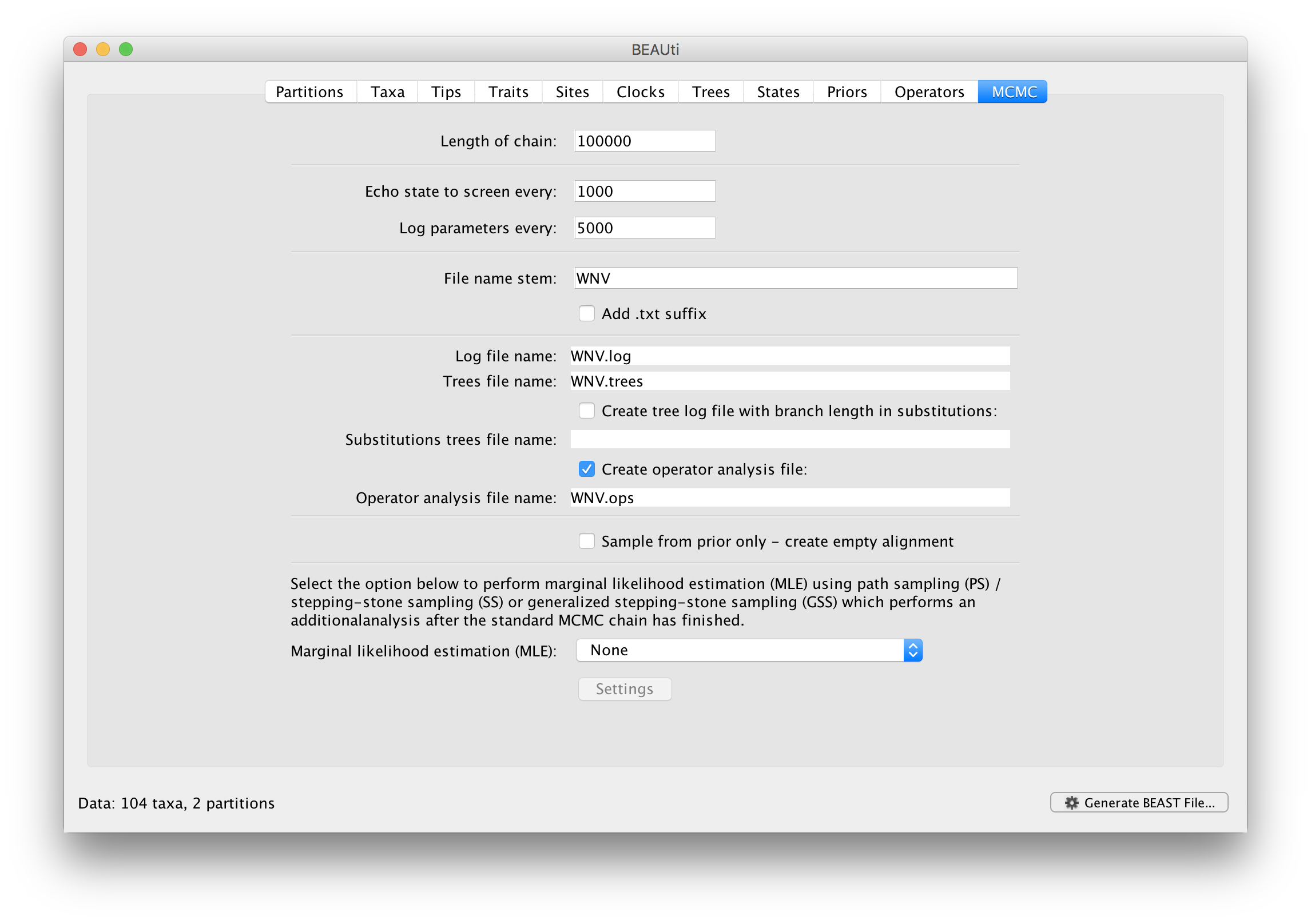
For this dataset let’s initially set the chain length to 100,000 as this will run reasonably quickly on most modern computers. Because the renaissance counting procedure, which is executed each time a state is logged, can be computationally expensive for a large coding sequence alignment, we will set the parameter logging to file to 5000 and the state echo to screen every 100 state.

The next option allows the user to set the File stem name; set this to ‘WNV_homogeneous’ (‘homogeneous’ for ‘homogeneous Brownian diffusion’). The next two options give the file names of the log files for the parameters and the trees. These will be set based on the file stem name. You can also log the operator analysis to a file. An option is also available to sample from the prior only, which can be useful to evaluate how divergent our posterior estimates are when information is drawn from the data. Here, we will not select this option, but analyze the actual data.

Finally, one can select to perform marginal likelihood estimation to assess model fit, which is not needed in this exercise. So, at this point we are ready to generate a BEAST XML file and to use this to run the Bayesian evolutionary analysis. To do this, either select the Generate BEAST File... option from the File menu or click the similarly labelled button at the bottom of the window. BContinue and choose a name for the file (for example, WNV_homogeneous.xml by adding the xml extension to the file name stem) and save the file. For convenience, you can leave the BEAUti window open so that you can change the values and re-generate the BEAST file if necessary.

Running BEAST

Once the BEAST XML file has been created the analysis itself can be performed using BEAST. The exact instructions for running BEAST depends on the computer you are using, but in most cases a dialog box will appear in which you select the XML file:

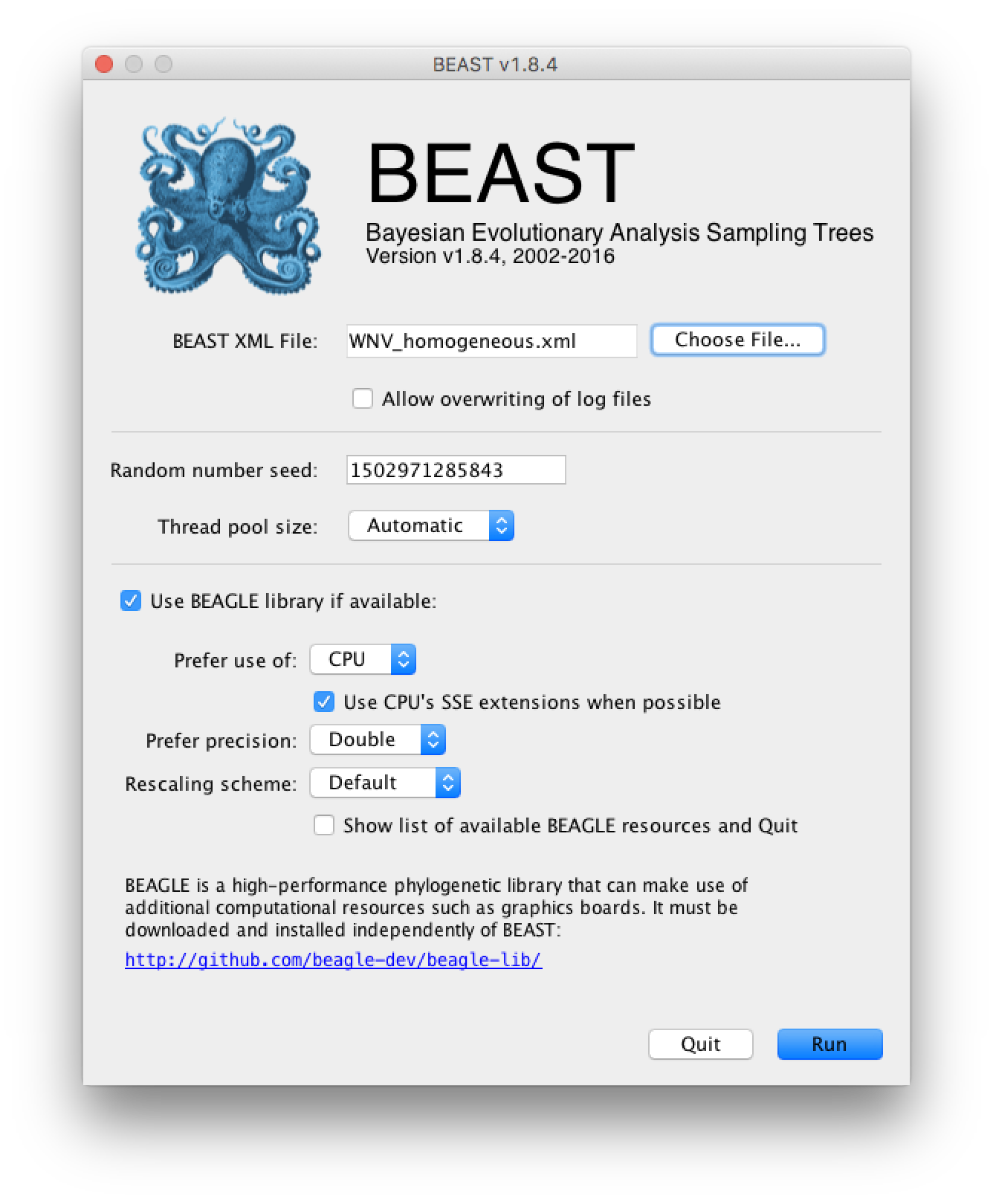
Press the ‘Choose File’ button and select the XML file you just created and press ‘Run’. When you have installed the BEAGLE library (https://github.com/beagle-dev/beagle-lib), you can use this in conjunction with BEAST to speed up the calculations. If not installed, unselect the use of the BEAGLE library. If the command line version of BEAST is being used then the name of the XML file is given after the name of the BEAST executable. The analysis will then be performed with detailed information about the progress of the run being written to the screen. When it has finished, the log file and the trees file will have been created in the same location as your XML file.

Analyzing the BEAST output

To analyze the results of running BEAST we are going to use the program Tracer. The exact instructions for running Tracer differs depending on which computer you are using. Double click on the Tracer icon; once running, Tracer will look similar irrespective of which computer system it is running on.

Select the Import Trace File... option from the File menu. If you have it available, select the log file that you created in the previous section (WNV_homogeneous.log). Alternative, drag and drop your log file into the Tracer window. The file will load and you will be presented with a window similar to the one below. Remember that MCMC is a stochastic algorithm so the actual numbers will not be exactly the same.

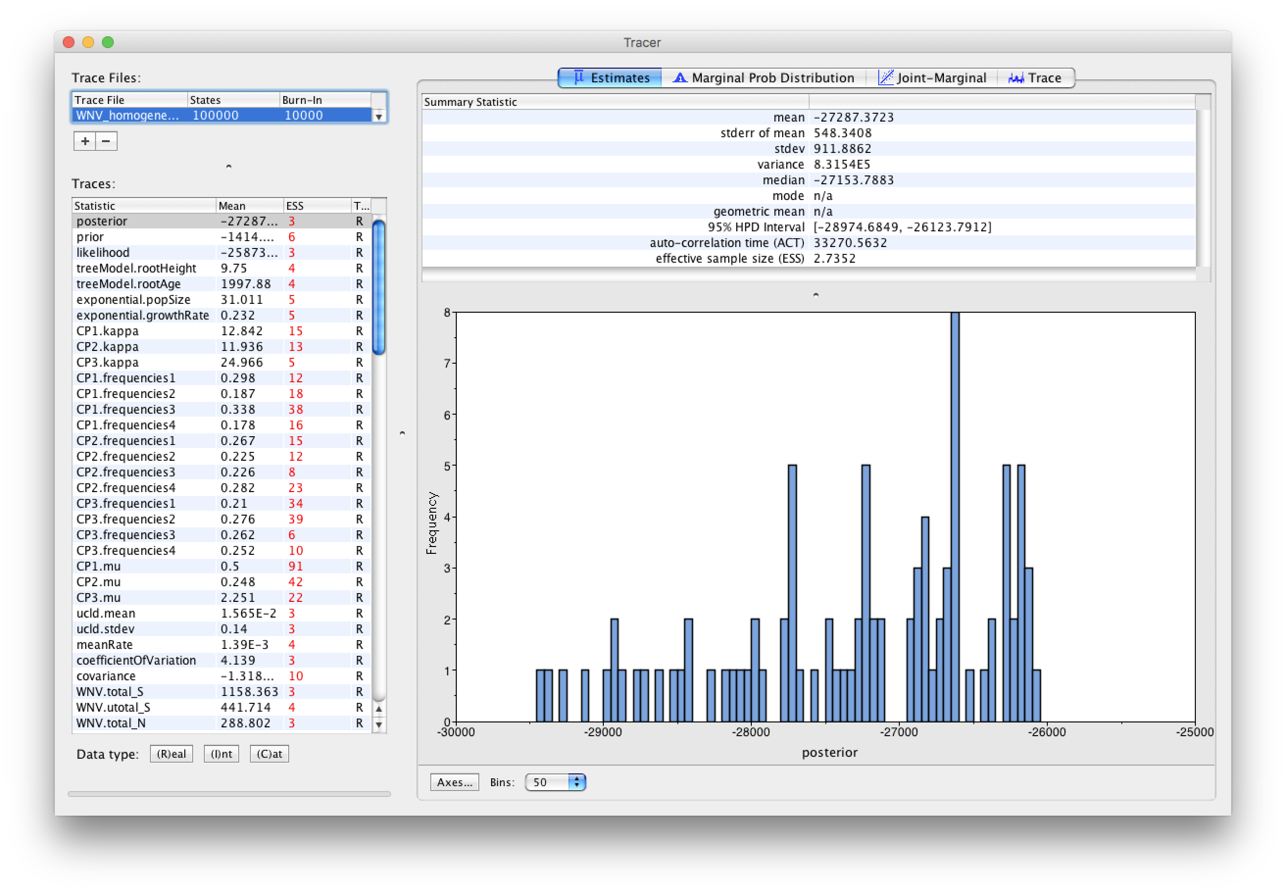
On the left hand side is the name of the log file loaded and the traces that it contains. There are traces for the posterior (this is the log of the product of the tree likelihood and the prior probabilities), and the continuous parameters. Selecting a trace on the left brings up analyses for this trace on the right hand side depending on tab that is selected. When first opened, the ‘posterior’ trace is selected and various statistics of this trace are shown under the Estimates tab.

In the top right of the window is a table of calculated statistics for the selected trace. The statistics and their meaning are described in the table below.

• Mean - The mean value of the samples (excluding the burn-in).
• Stdev - The standard error of the mean. This takes into account the effective sample size so a small ESS will give a large standard error.
• Median - The median value of the samples (excluding the burn-in).
• 95% HPD Lower - The lower bound of the highest posterior density (HPD) interval. The HPD is the shortest interval that contains 95% of the sampled values.
• 95% HPD Upper - The upper bound of the highest posterior density (HPD) interval.
• Auto-Correlation Time (ACT) - The average number of states in the MCMC chain that two samples have to be separated by for them to be uncorrelated (i.e. independent samples from the posterior). The ACT is estimated from the samples in the trace (excluding the burn-in).
• Effective Sample Size (ESS) - The effective sample size (ESS) is the number of independent samples that the trace is equivalent to. This is calculated as the chain length (excluding the burn-in) divided by the ACT.

Note that the effective sample sizes (ESSs) for all the traces are small (ESSs less than 100 are highlighted in red by Tracer and values > 100 but < 200 are in yellow). This is not good. A low ESS means that your samples are equivalent to only few uncorrelated samples trace and this may not represent the posterior distribution well. In the bottom right of the window is a frequency plot of the samples which is expected given the low ESSs is extremely rough. Inspecting the Trace of many continuous parameters shows that the chain is still in the burn-in phase (the posterior values are still increasing over the entire chain), and this run does not allow us to summarize marginal posterior probability distributions for the parameters.

The simple response to this situation is that we need to run the chain for longer.

For this exercise, output files from longer runs are made available:

Import the log file for the long run of the homogenous model and reassure yourself that the MCMC run has reached stationarity: there are no obvious trends in the plot which would suggest that the MCMC has not yet converged, and there are no large-scale fluctuations in the trace which would suggest poor mixing.

As we are happy with the behavior of posterior probability we can now move on to our statistic of interest: the dispersion rate. Select ‘location.diffusionRate’ in the left-hand table. This shows a plot of the posterior probability density of this statistic that keeps track of the rate of diffusion by measuring the distance covered along each branch (based on the spatial coordinates inferred at the parent and descendent node of each branch), summing this distance for the complete tree and dividing this by the tree length. It uses the great circle distance between the two coordinates, which will provide an estimate in km/yr. You should see a plot similar to this in the Estimates tab:

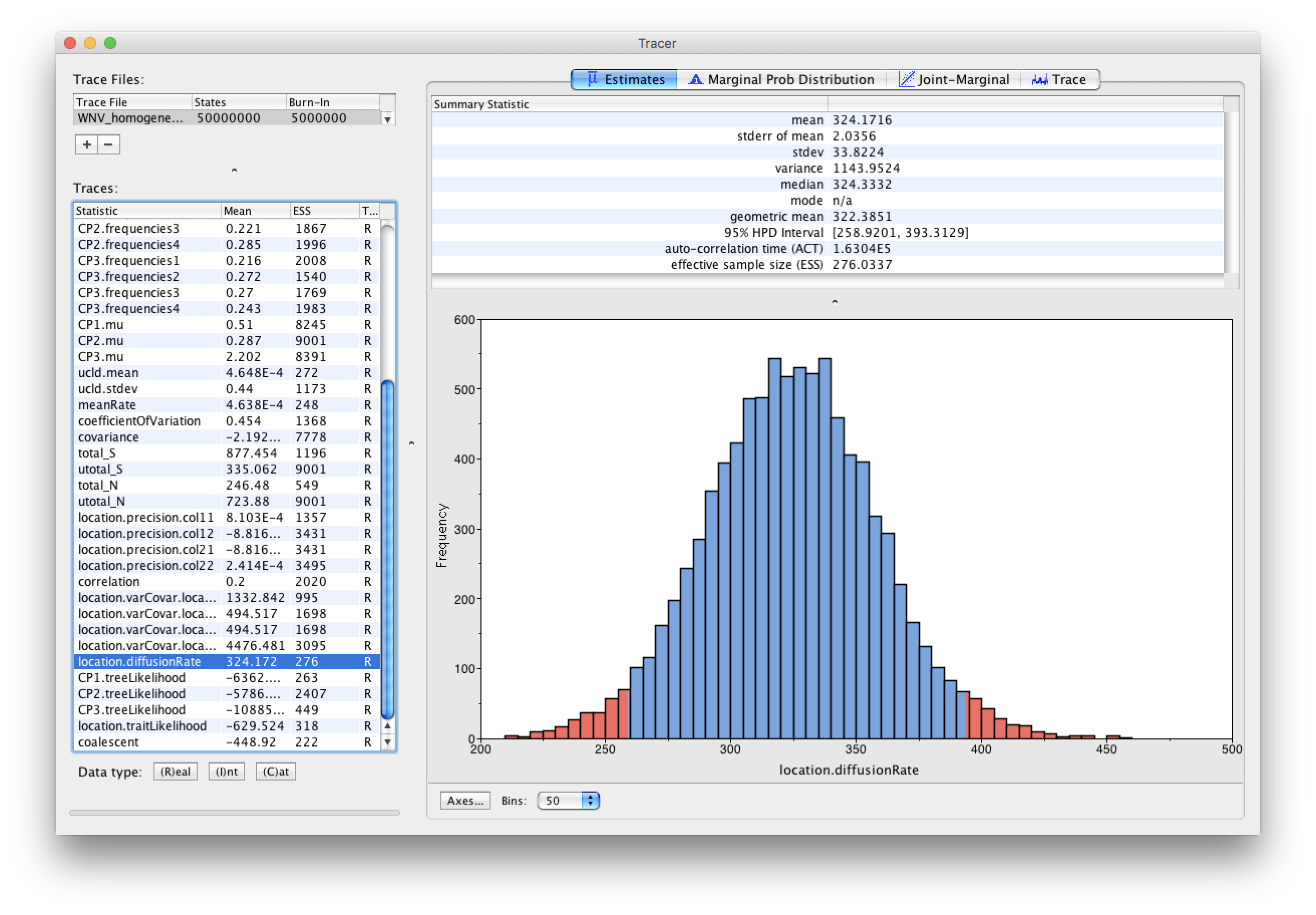
At what rate has WNV invaded North America?

Summarizing the trees

We have seen how we can diagnose our MCMC run using Tracer and produce estimates of the marginal posterior distributions of parameters of our model. However, BEAST also samples trees (either phylogenies or genealogies) at the same time as the other parameters of the model. These are written to a separate file called the ‘trees’ file. This file is a standard NEXUS format file. As such it can easily be loaded into other software in order to examine the trees it contains. One possibility is to load the trees into a program such as PAUP* and construct a consensus tree in a similar manner to summarizing a set of bootstrap trees. In this case, the support values reported for the resolved nodes in the consensus tree will be the posterior probability of those clades.

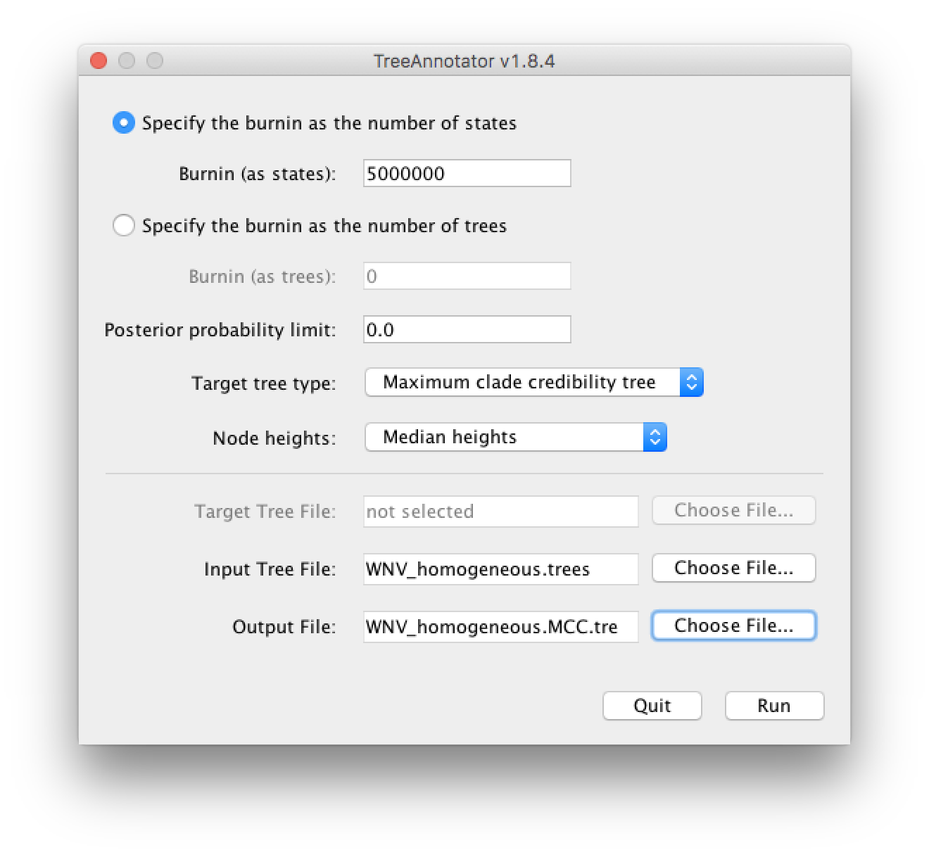
In this tutorial, however, we are going to use a tool that is provided as part of the BEAST package to summarize the information contained within our sampled trees. The tool is called TreeAnnotator and once running, you will be presented with a window like the one below.

• TreeAnnotator takes a single ‘target’ tree and annotates it with the summarized information from the entire sample of trees. The summarized information includes the average node ages (along with the HPD intervals), the posterior support and the average rate of evolution on each branch (for relaxed clock models where this can vary). The program calculates these values for each node or clade observed in the specified ‘target’ tree. It has the following options:

• Burnin - This is the number of steps in the MCMC chain, Burnin (as states), or the number of trees, Burnin (as trees), that should be excluded from the summarization. For the example above, with a chain of 200,000,000 steps, a 10% burnin corresponds to 20,000,000 steps. Alternatively, sampling every 50,000 steps results in 4000 trees in the file, and to obtain at the same 10% burnin, the number of trees needs to be set to 400.

• Posterior probability limit - This is the minimum posterior probability for a node in order for TreeAnnotator to store the annotated information. The default is 0.0 so every node, no matter what its support, will have information summarized. Make sure this value remains 0.0 as every node will require location annotation for further visualization.

• Target tree type - This has three options Maximum clade credibility tree or User target tree For the latter option, a NEXUS tree file can be specified as the Target Tree File, below. Select the first option, TreeAnnotator will examine every tree in the Input Tree File and select the tree that has the highest product of the posterior probabilities of all its nodes.

• Node heights - This option specifies what node heights (times) should be used for the output tree. If the Keep target heights is selected, then the node heights will be the same as the target tree. Node heights can also be summarised as a Mean or a Median over the sample of trees. Sometimes a mean or median height for a node may actually be higher than the mean or median height of its parental node (because particular ancestral-descendent relationships in the MCC tree may still be different compared to a large number of other tree sampled). This will result in artifactual negative branch lengths, but can be avoided by the Common Ancestor heights option. Let’s use the default Median heights for our summary tree.

• Target Tree File - If the User target tree option is selected then you can use Choose File... to select a NEXUS file containing the target tree.

Input Tree File - Use the Choose File... button to select an input trees file. This will be the trees file produced by BEAST.

• Output File - Select a name for the output tree file (e.g., ‘WNV_homogeneous.tre’).

Once you have selected all the options, above, press the Run button. TreeAnnotator will analyse the input tree file and write the summary tree to the file you specified. This tree is in standard NEXUS tree file format so may be loaded into any tree drawing package that supports this. However, it also contains additional information that can only be displayed using the FigTree program.

Viewing the annotated tree

Run FigTree and select the Open... command from the File menu. Select the tree file you created using TreeAnnotator in the previous section. The tree will be displayed in the FigTree window. On the left hand side of the window are the options and settings which control how the tree is displayed. In this case we want to display the posterior probabilities of each of the clades present in the tree and estimates of the age of each node. In order to do this you need to change some of the settings.

First, re-order the node order by Increasing Node Order under the Tree Menu. Click on Branch Labels in the control panel on the left and open its section by clicking on the arrow on the left. Now select ‘posterior’ under the Display popup menu. The posterior probabilities won’t actually be displayed until you tick the check-box next to the Branch Labels title.

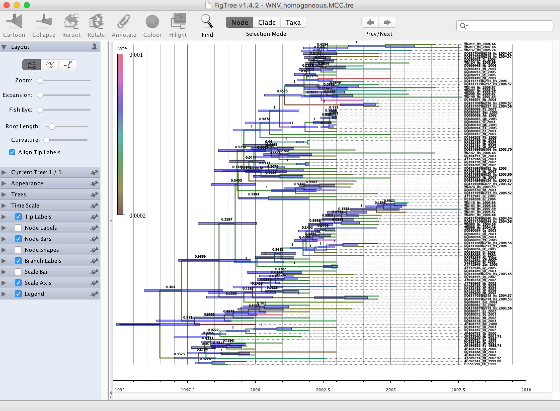
We now want to display bars on the tree to represent the estimated uncertainty in the date for each node. TreeAnnotator will have placed this information in the tree file in the shape of the 95% highest posterior density (HPD) intervals (see the description of HPDs, above). Select Node Bars in the control panel and open this section; select height_95%_HPD to display the 95% HPDs of the node heights. We can also plot a time scale axis for this evolutionary history (select Scale Axis and deselect Scale bar). For appropriate scaling, open the Time Scale section of the control panel, set the Offset to 2007.63 (date of the most recent sample), and select Reverse Axis under Scale Axis.

In the Layout panel select the check-box Align Tip Labels to increase clarity.

Finally, open the Appearance panel and alter the Line Weight to draw the tree with thicker lines. Under the same panel, alter Colour by and select ‘rate’. Select the Legend option and choose ‘rate’ as an attribute to display a legend for the branch coloring. None of the options actually alter the tree’s topology or branch lengths in anyway so feel free to explore the options and settings. You can also save the tree and this will save all your settings so that when you load it into FigTree again it will be displayed exactly as you selected.

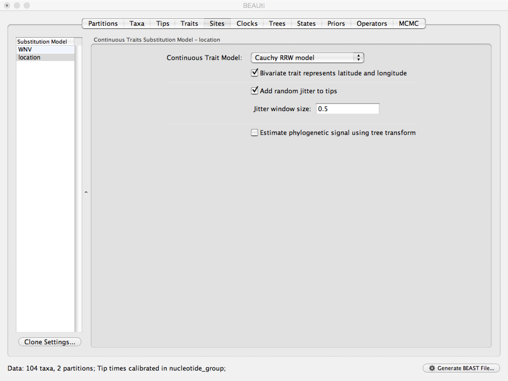
Evaluating diffusion rate variation

To investigate whether the rate of spread was roughly constant throughout the rabies epidemic we can fit models that allow for branch-specific rate variation in the diffusion process (termed ‘relaxed random walks’, RRWs) and test whether these result in a model fit improvement compared to the standard homogeneous Brownian diffusion process. To this purpose, we have also analyzed the same data under a ‘Cauchy RRW’. This can be set under the Sites tab for the ‘location’ Substitution model:

For the different models, we can estimate marginal likelihoods (MLE) using path sampling (PS) and stepping stone sampling, which have recently been implemented in BEAST (Baele at al., 2012, 2013). Typically, PS/SS model selection is performed after doing a standard MCMC analysis. PS and SS sampling can then start where the MCMC analysis has stopped (i.e. you should have run the MCMC analysis long enough so that it has converged towards the posterior before attempting a PS/SS analysis), thereby eliminating the need for PS and SS to first converge towards the posterior. To set up such analyses, we can return to BEAUti and select ‘path sampling (PS) / stepping-stone sampling (SS)’ from the Perform marginal likelihood estimation (MLE) menu, which performs an additional analysis after the standard MCMC chain has finished. In the MCMC panel, Click on settings to specify the PS/SS settings.

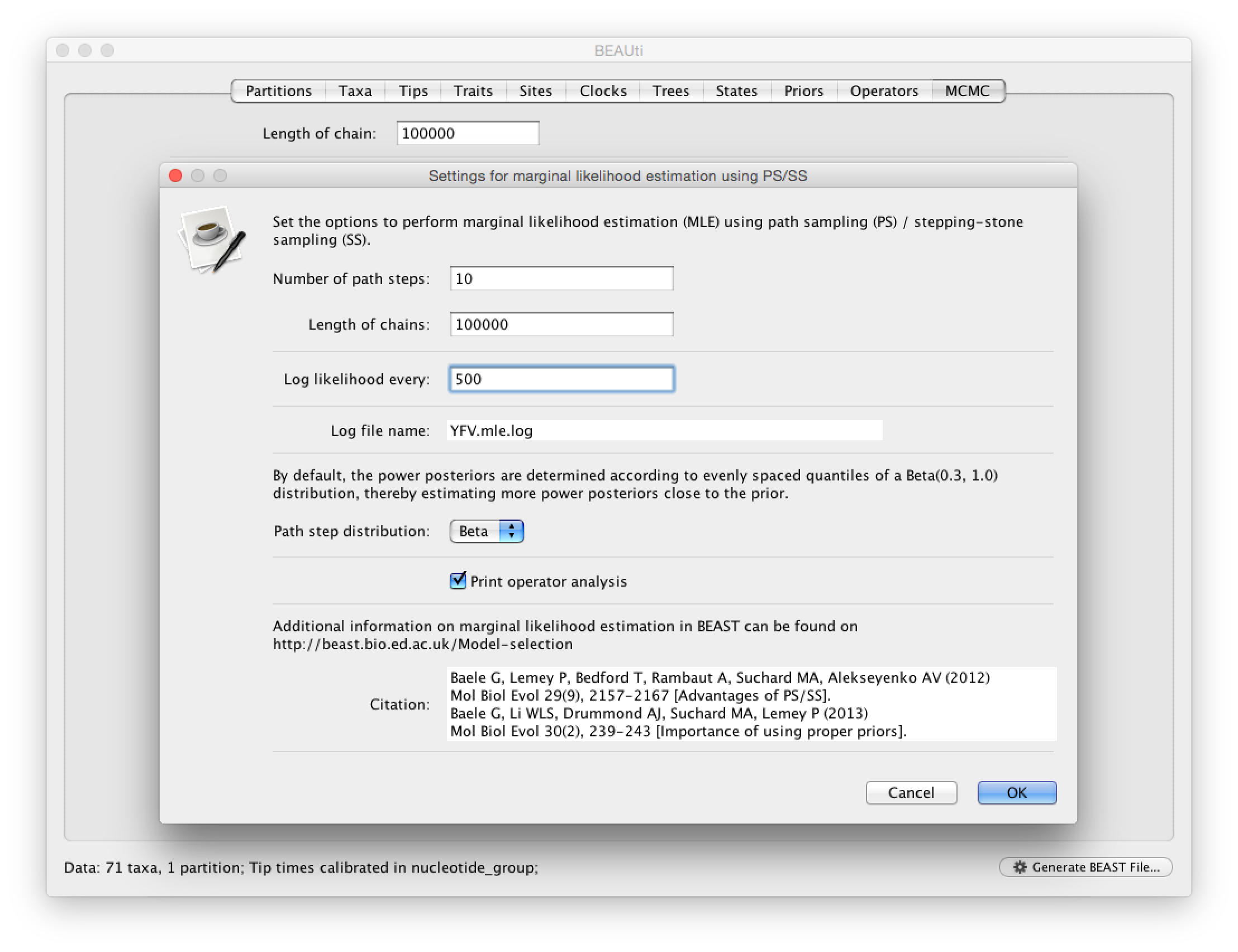
We need to set the number of steps (in this case 50) for the path between the posterior and the prior, the length of the MCMC chain (in this case 1,000,000) for each step that estimates a specific power posterior, and the logging frequency for each MCMC sampling (in this case every 1,000). Note that using these settings, the marginal likelihood estimation will take approximately the time it takes to complete a standard MCMC run of 50,000,000 generations for this data. The powers for the different power posteriors are defined using evenly spaced quantiles of a Beta(\alpha,1.0) distribution, with α here equal to 0.30, as suggested in the stepping-stone sampling paper (Xie et al. 2011) since this approach is shown to outperform a uniform spreading suggested in the path sampling paper (Lartillot and Philippe 2006). Note that a more recently developed marginal likelihood estimator, i.e. generalised stepping-stone sampling (Fan et al., 2011; Baele et al., 2016), is now availble, but this has not been tested yet for the comparison of trait diffusion models.

Based on the settings above, the homogeneous Brownian analysis results in marginal likelihood estimates of -24182.20 and -24176.83 for PS and SS respectively. For the Cauchy RRW, we get -24074.30 and -24072.10 for the same estimators. Is there significant evidence for diffusion rate heterogeneity? Does this have a big effect on the mean dispersal rate estimate? The rate variation among lineages can be depicted in the MCC tree using a colour annotation. Summarize the MCC tree for the Cauchy RRW model and under Appearance in FigTree, select to Colour by ‘location.rate’.

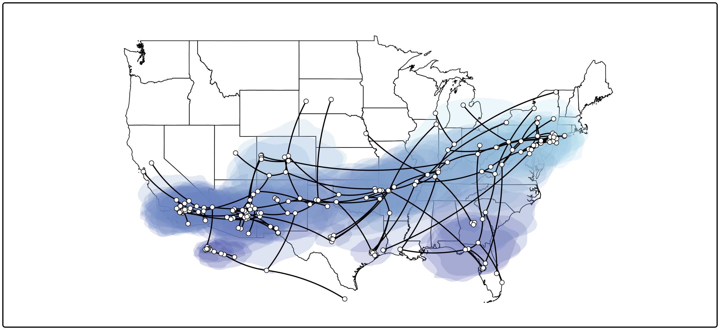
Visualizing Bayesian phylogeographic reconstructions using SpreaD3

SpreaD3, i.e. Spatial Phylogenetic Reconstruction of EvolutionAry Dynamics using Data-Driven Documents (D3), is a software to visualize the output from Bayesian phylogeographic analysis and constitutes a user-friendly application to analyze and visualize pathogen phylodynamic reconstructions resulting from Bayesian inference of sequence and trait evolutionary processes. SpreaD3 allows to visualise on custom maps and generates HTML pages for display in modern-day browsers such as Firefox, Safari and Chrome. One of the functionalities of SpreaD3 that relate to the continuous phylogeographic analysis performed previously include visualizing location-annotated MCC trees. A detailed tutorial for this particular step is available here. Brief instructions can be found in the quick how-to summary below. Compare the animated version for both the homogeneous and RRW model: do you notice any difference?

Quantifying site-specific selection using dN/dS estimates

As part of our WNV analysis, we performed a ‘Renaissance Counting’ procedure to obtain site-specific dN/dS estimates. These estimates are logged in the WNV_homogeneous.dNdS.log file and summarized in WNV_homogeneous.dNdS.summary.txt. In this summary, each codon site is listed with its mean dN/dS estimate and credible intervals (CPD Low and CPD Up). In addition, a classification is provided based on these estimates according to three categories: negatively selected represented by ‘-’, neutral, represented by ‘0’ and positively selected represented by ‘+’. Finally, when sites are considered to be significantly negatively or positively selected (based in the frequency by which 1 is covered by the credible intervals of the dN/dS estimate), this is indicated with a ‘*’. In general, the mean dN/dS estimates are low and the variation in their values is fairly discrete. This is due to the sparsity of the number of substitutions in this data, in particular nonsynonymous substitutions. So negative selection is the dominating evolutionary force in the WNV history. There are however five sites that are estimated to be under (not so strong) positive selection (449, 1367, 1991, 2209, 2518, 2522 and 2842). Were any of these sites also detected to be positively selected in the this study?

A quick how-to summary

Run BEAUti

• Load a NEXUS format alignment by selecting the Import Data... option from the File menu. Select the file called ‘WNV.fas’.

• In the Tips tab, select the Use tip dates option and use the Parse Dates button. Keep the default Defined just by its order, set order to last, and Parse as a number: add the following value to each: 1900.0, …unless less than 16.0, … in which case add: 2000.0. Select all the taxa (holding down the cmd key) with sampling dates only known up to the year in the Tips window (those with a .0 decimal) and click on Set Uncertainty. Enter ‘1.0’ as the precision value for 1 year. Select sampling uniformly from uncertainty at the bottom left of the Tips panel and keep the Apply to taxon set: All taxa default.

• In the Traits tab, click Import trait. Browse to and load the WNV_lat_long.txt tab-delimited file

• After loading the file, select both the ‘Lat’ and ‘Long’ traits in the panel on the left and select Create partition from trait... Enter the name ‘location’ for this partition:

• In the Sites tab, keep the default HKY substitution model, keep the base frequencies to be Estimated, the ‘Site Rate Heterogeneity’ to ‘None’, and partition the data into 3 partitions for the coding positions (3 partitions: positions 1,2,3).

• Click on location in the Substitution model window on the left and keep the default ‘Homogenous Brownian model’ and select Bivariate trait represents latitude and longitude and a Jitter set to ‘0.5’.

• In the Clocks tab, select the Lognormal relaxed molecular clock (Uncorrelated) model.

• In the Trees tab, select the exponential growth model as the demographic tree prior (Coalescent: Exponential Growth) and keep the default random starting tree.

• In the States tab, turn on the Renaissance counting procedure by selection Reconstruct synonymous/non-synonymous change counts In the Priors tab, set the allMus prior to a lognormal distribution with mean = 0.0 and stdev = 1.5.

• In the MCMC tab, set the chain length to 100,000 and both the sampling frequencies to 5000. Set the File name stem to ‘WNV_homogeneous’ and generate the beast file (‘WNV_homogeneous.xml’).

Run BEAST and load the xml file.

Analyze the output using Tracer. Analyze the output file for the longer runs.

Summarize the trees for the longer run using treeAnnotator.

Visualize the tree in FigTree.

Run SpreaD3.

We will first summarise an MCC tree and then summarise the information in the entire tree distribution.

• Select as input type in the Data panel: MCC tree with CONTINUOUS traits, load your MCC tree file.

• Select ‘location1’ as Latitute attribute name and ‘location2’ as Longitude attribute name.

• Set the most recent sampling date to 2007-07-15.

• Load a GeoJSON file of the United States.

• Keep all other default settings and click Output to generate a JSON file.

• Go to the Rendering panel, keep the D3 renderer as the renderer of choice, and load the generated JSON file.

• Click Render to D3 to generate the HTML page and a browser window will open automatically.

This visualizes the MCC tree an the uncertainty for its node locations. To summarize the location uncertainty based on the entire tree distribution we can continue with the following procedure.

• Select as input type in the Data panel: Tree distribution with CONTINUOUS traits, load your ‘.trees’ file.

• Keep the default Time slices (Generated from MCC tree) and load this MCC tree.

• Set the most recent sampling date to 2007-07-15.

• Set the 2D rate attribute to ‘location.rate’.

• Keep all other default settings and click Output to generate a JSON file.

• Go to the Merge panel and choose the JSON that you have just created. Add a second line using the + button in the lower left corner. Choose the MCC tree JSON file.

• Select the Areas from the first JSON file and the Points, Lines and GeoJSON from the second (MCC tree) JSON file.

• Select Merge... from the File menu and save the new merged JSON.

• Go to the Rendering panel, keep the D3 renderer as the renderer of choice, and load the generated JSON file.

• Click Render to D3 to generate the HTML page and a browser window will open automatically.

Conclusion and Resources

This tutorial only scratches the surface of the analyses that are possible to undertake using BEAST. It has hopefully provided a relatively gentle introduction to the fundamental steps that will be common to all BEAST analyses and provide a basis for more challenging investigations. BEAST is an ongoing development project with new models and techniques being added on a regular basis. The BEAST website provides details of the mailing list that is used to announce new features and to discuss the use of the package. The website also contains a list of tutorials and recipes to answer particular evolutionary questions using BEAST as well as a description of the XML input format, common questions and error messages.

References

• Lemey, P., A. Rambaut, J. J. Welch, and M. A. Suchard. 2010. Phylogeography takes a relaxed random walk in continuous space and time. Molecular biology and evolution 27:1877-1885.

• Pybus, O. G., M. A. Suchard, P. Lemey, F. J. Bernardin, A. Rambaut, F. W. Crawford, R. R. Gray, N. Arinaminpathy, S. L. Stramer, M. P. Busch, and E. L. Delwart. 2012. Unifying the spatial epidemiology and molecular evolution of emerging epidemics. Proceedings of the National Academy of Sciences of the United States of America 109:15066-15071.

• Baele, G., P. Lemey, T. Bedford, A. Rambaut, M. A. Suchard, and A. V. Alekseyenko. 2012. Improving the accuracy of demographic and molecular clock model comparison while accommodating phylogenetic uncertainty. Molecular biology and evolution 29:2157-2167.

• Baele, G., W. L. Li, A. J. Drummond, M. A. Suchard, and P. Lemey. 2013. Accurate model selection of relaxed molecular clocks in bayesian phylogenetics. Molecular biology and evolution 30:239-243.

• Baele, G., P. Lemey, M. A. Suchard. 2016. Genealogical working distributions for Bayesian model testing with phylogenetic uncertainty. Systematic biology 65:250-264.

• Lemey, P., V. N. Minin, F. Bielejec, S. L. Kosakovsky Pond, and M. A. Suchard. 2012. A counting renaissance: Combining stochastic mapping and empirical Bayes to quickly detect amino acid sites under positive selection. Bioinformatics 28(24):3248–3256.

• Bielejec, F., G. Baele, B. Vrancken, M. A. Suchard, A. Rambaut and P. Lemey. 2016. SpreaD3: interactive visualisation of spatiotemporal history and trait evolutionary processes. Mol. Biol. Evol., 33(8): 2167–2169. doi: 10.1093/molbev/msw082