Introduction
The first step will be to convert a NEXUS file with a DATA or CHARACTERS block into a BEAST XML input file. This is done using the program BEAUti (this stands for Bayesian Evolutionary Analysis Utility). This is a user-friendly program for setting the evolutionary model and options for the MCMC analysis. The second step is to actually run BEAST using the input file that contains the data, model and settings. The final step is to explore the output of BEAST in order to diagnose problems and to summarize the results.
To undertake this tutorial, you will need to download three software packages in a format that is compatible with your computer system (all three are available for Mac OS X, Windows and Linux/UNIX operating systems):
Running BEAUti
To load a NEXUS format alignment, simply select the Import NEXUS... option from the File menu.
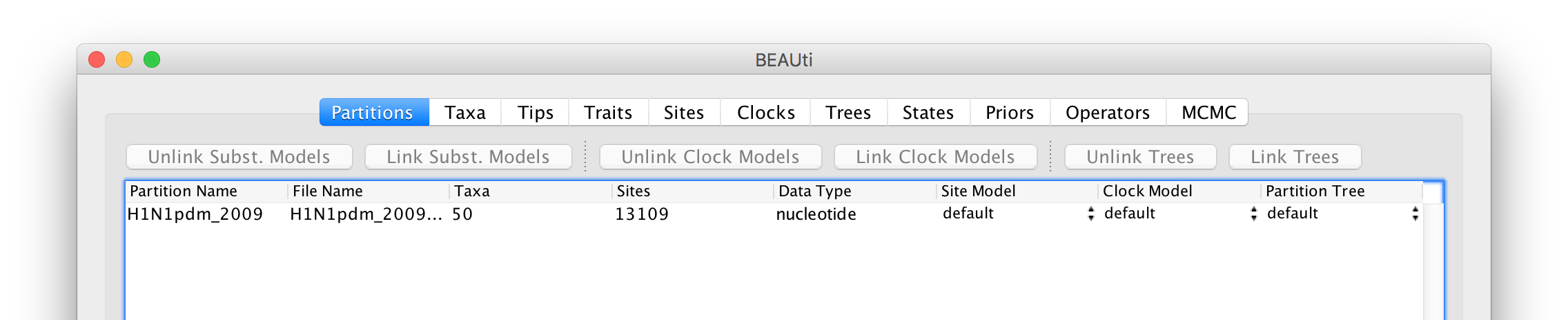
Select the file called H1N1pdm_2009.nex. This file contains an alignment of 50 genomes (all 8 genomic segments concatinated), 13109 nucleotides in length. Once loaded, the new data will be listed under Partitions as shown in the figure:
Setting the tip dates
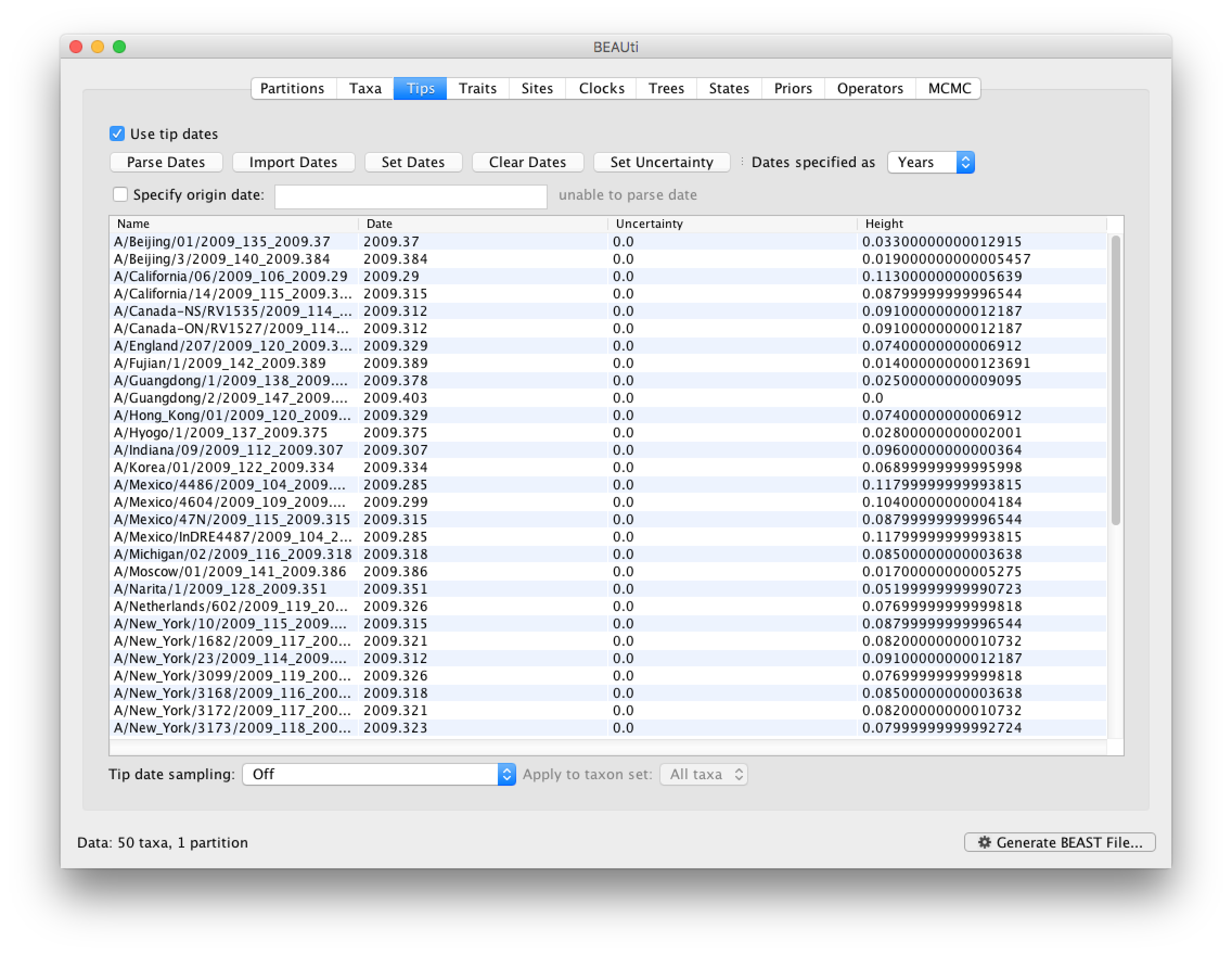
To undertake a phylodynamic analysis we need to specify the dates that the individual viruses were collected. In this case, the sequences were sampled from the H1N1 2009 pandemic between March and May 2009. To set these dates switch to the Tips panel using the tabs at the top of the window.
Select the box labelled Use tip dates. The actual sampling time in fractional years is encoded in the name of each taxon and we can use the Parse Dates button at the top of the panel to extract these. For the H1N1pdm_2009 sequences you can keep the default Defined just by its order and select last from the drop-down menu for the order and press OK. The dates will appear in the appropriate column of the main window. You can then check these and edit them manually as required.
Setting the substitution model
The next thing to do is to click on the Sites tab at the top of the main window to specify the evolutionary model settings for BEAST:
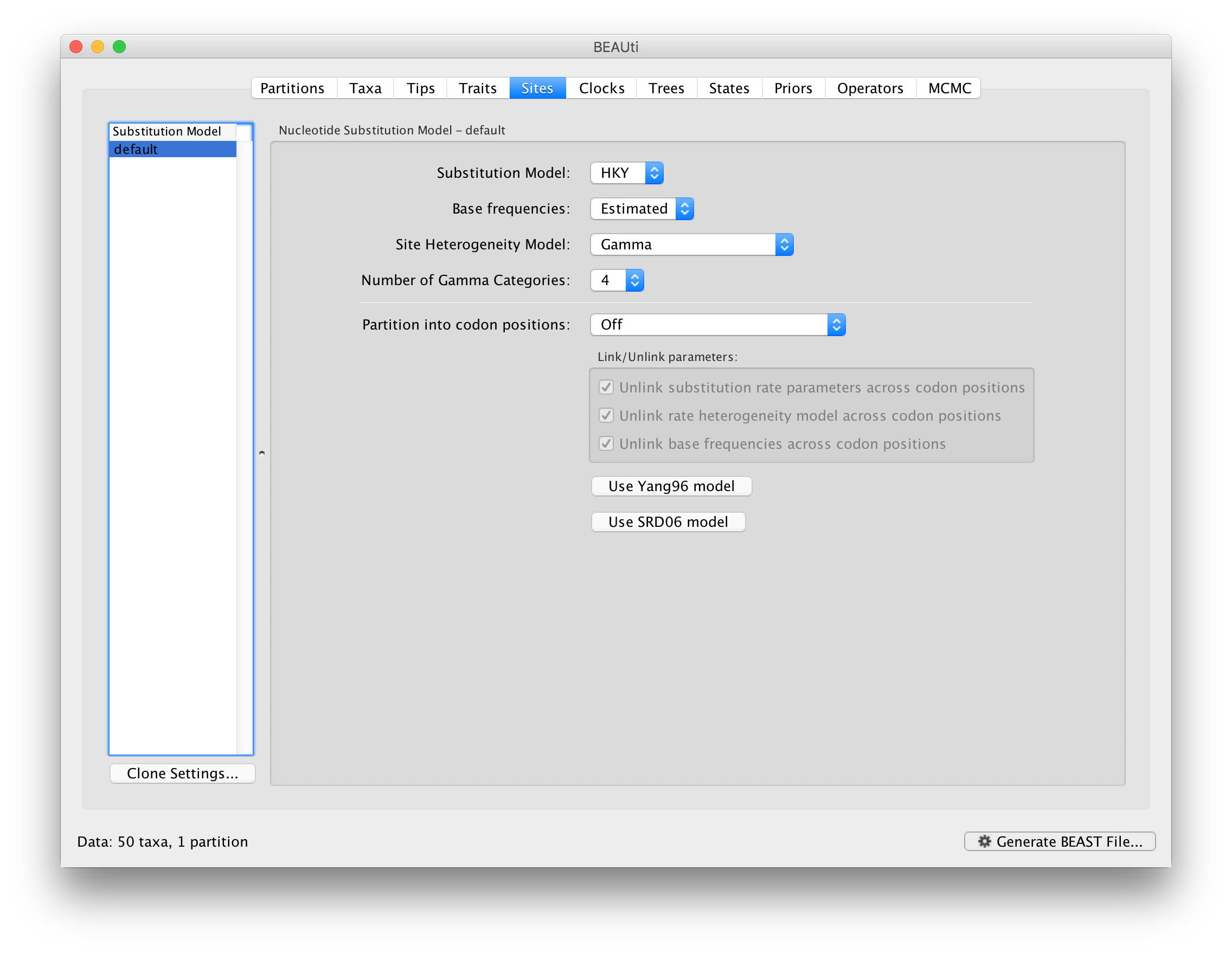
For this tutorial, keep the default HKY model, the default Estimated base frequencies and select Gamma as Site Heterogeneity Model (with 4 discrete categories) before proceeding to the Clocks tab.
Setting the molecular clock model
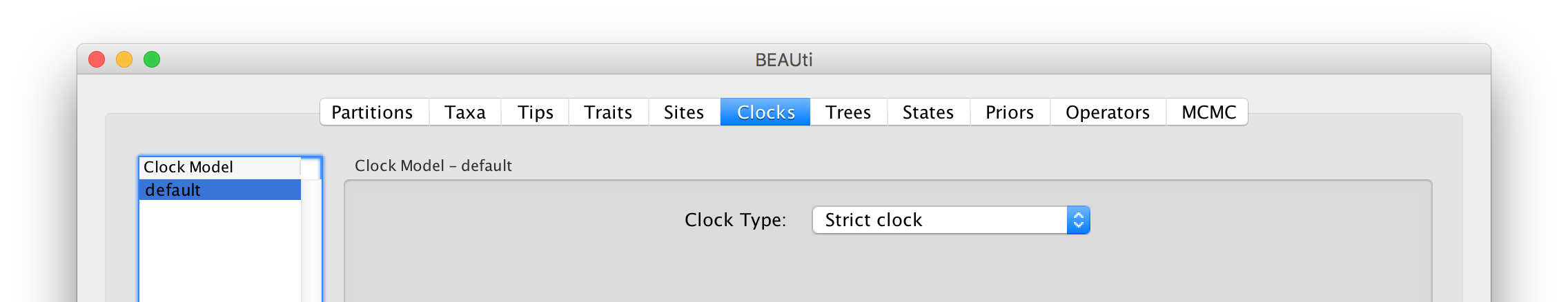
The Clock panel options allows us to choose between a strict and a relaxed (uncorrelated lognormal or uncorrelated exponential) clock. Because of the low diversity data we analyze here, a relaxed clock would probably be over-parameterization. Hence, we keep a strict clock setting.
Now move on to the Trees panel.
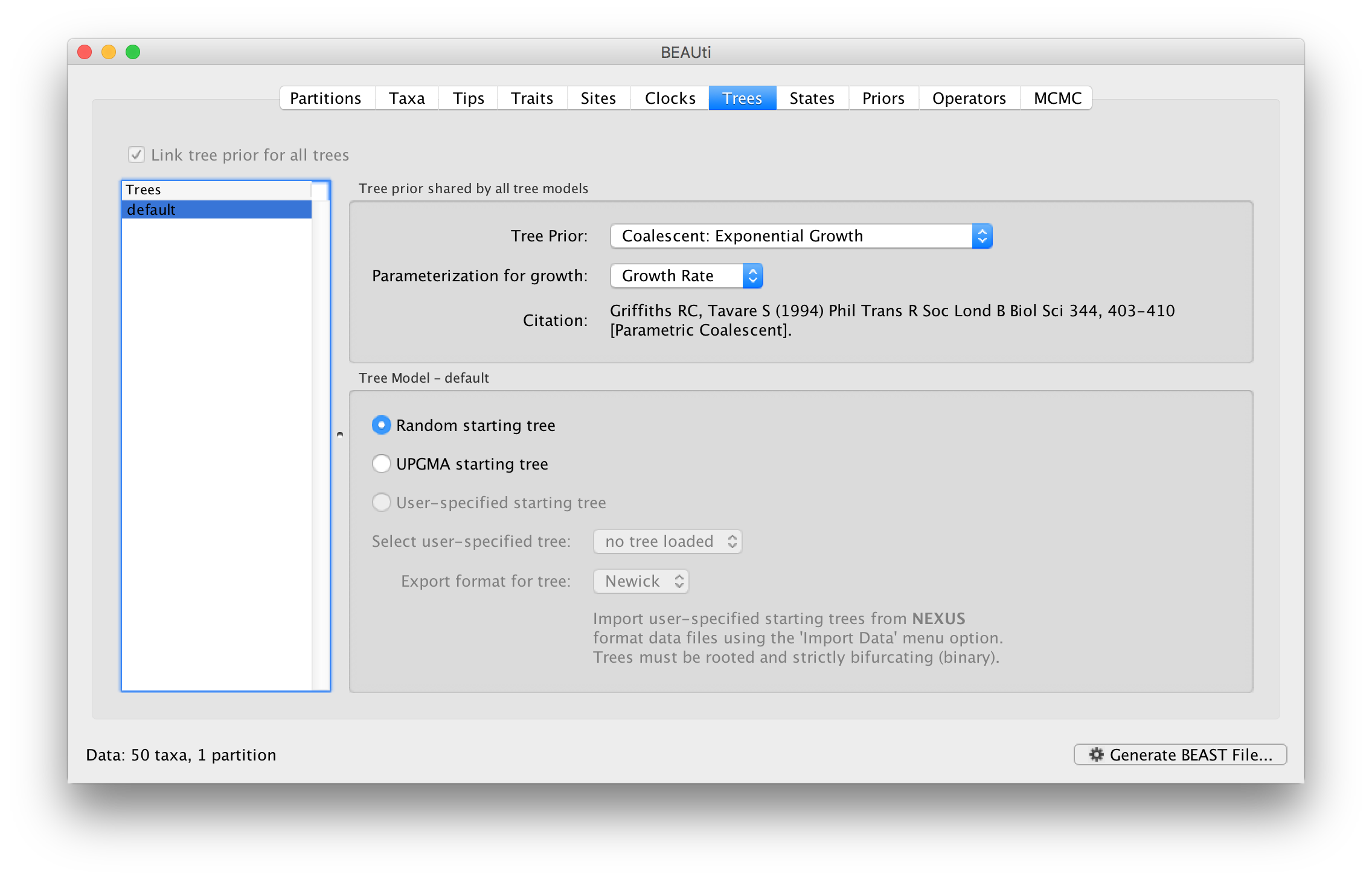
Setting the tree prior
This panel contains settings about the tree. Firstly the starting tree is specified to be ‘randomly generated’. The other main setting here is to specify the ‘Tree prior’ which describes how the population size is expected to change over time for coalescent models. The default tree prior is set to a constant size coalescent prior. The range of different tree priors (coalescent and other models) are described on this page.
To estimate the epidemic growth rate, we will change this demographic model to an exponential growth coalescent prior, which is intuitively appealing for viral outbreaks. Switch the option for Tree Prior to Coalescent: Exponential Growth:
Setting up the priors
Now switch to the Priors tab. This panel has a table showing every parameter of the currently selected model and what the prior distribution is for each. A strong prior allows the user to ‘inform’ the analysis by selecting a particular distribution with a small variance. Alternatively we can select a weak (diffuse) prior to try to minimise the effect on the analysis. Note that a prior distribution must be specified for every parameter and whilst BEAUti provides default options these are not necessarily tailored to the problem and data being analyzed.
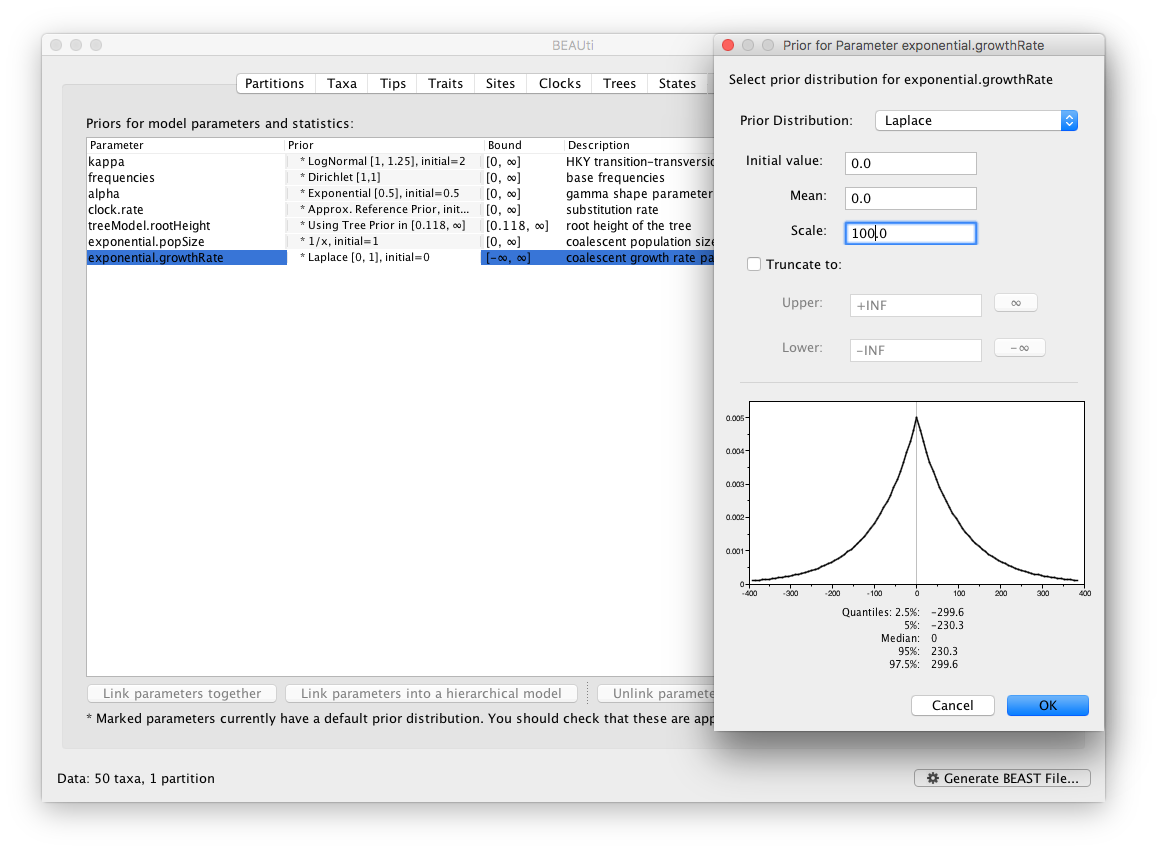
In this case, the default prior for the exponential growth rate (the Laplace distribution) prefers relatively small growth rates because the of the default scale (1.0). However, on this epidemic scale, the growth rate parameter take could take on relatively large values. Therefore, we will increase the variance of this prior distribution by setting the scale to 100. A useful exercise could be to examine the sensitity of the growth rate estimates to different scale values for this prior distribution (e.g. scale = 1, 10, 100).
The other priors can be left at their default options.
Setting up the operators
Each parameter in the model has one or more “operators” (these are variously called moves, proposals or transition kernels by other MCMC software packages such as MrBayes and LAMARC). The operators specify how the parameters change as the MCMC runs. The Operators tab in BEAUti has a table that lists the parameters, their operators and the tuning settings for these operators:
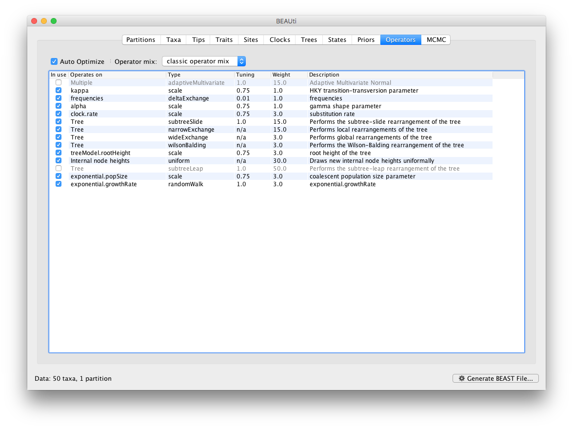
Notice that the coalescent growth rate parameter (exponential.growthrate) has a randomWalk operator. This is appropriate for a parameter that can take both positive and negative values (parameters that are strictly positive can use a scale operator). No changes are required in this table.
Setting the MCMC options
The MCMC tab in BEAUti provides settings to control the MCMC chain and the log files that get produced.
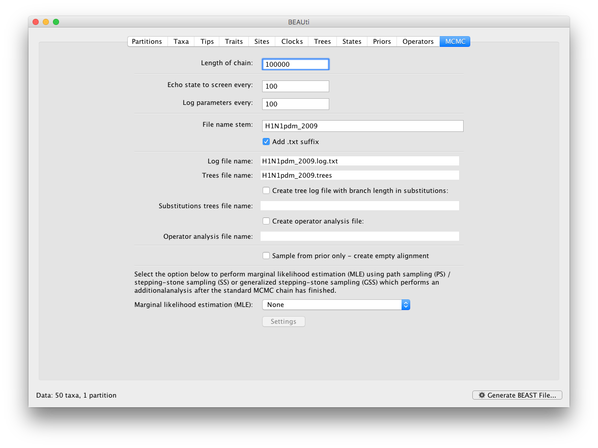
For this dataset let’s initially set the chain length to 100,000 and both the sampling frequencies to 100. The File name stem: should already be set to H1N1pdm_2009 but you can adjust this (perhaps add more indications about the analysis).
We are now ready to create the BEAST XML file. Select Generate XML... from the File menu (or the button at the bottom of the window). BEAUti will ask you to review the prior settings one more time before saving the file (and will indicate if any are improper). Continue and choose a name for the file — it will offer the name you gave it in the MCMC panel and we usually end the filename with ‘.xml’ (although on Windows machines you may want to give the file the extension ‘.xml.txt’).
Running BEAST
Once the BEAST XML file has been created the analysis itself can be performed using BEAST.
Once BEAST has started a dialog box will appear in which you select the XML file:
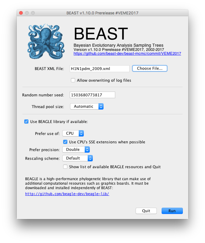
Press the Choose File... button and select the XML file you just created and press Run. The analysis will then be performed with detailed information about the progress of the run being written to the screen. When it has finished, the log file and the trees file will have been created in the same location as your XML file.
For more information about the other options in the BEAST dialog box see this page.
Analyzing the BEAST output
Select the Import Trace File... option from the File menu. Select the log file, H1N1pdm_2009.log, that you created in the previous section. The file will load and you will be presented with a window similar to the one below.
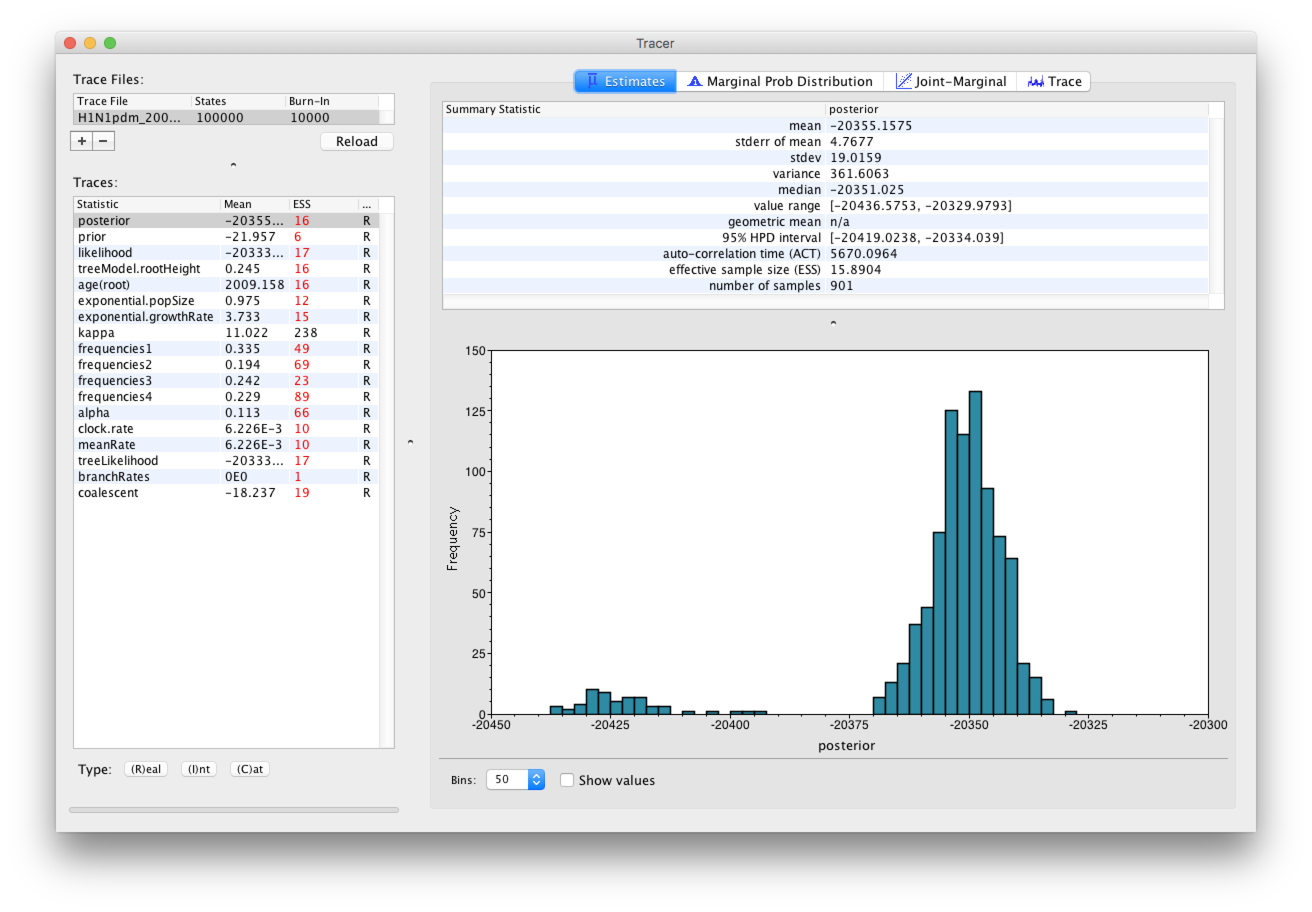
Similarly to the previous tutorial the effective sample sizes (ESSs) for all the traces are small (ESSs less 100 are highlighted in red respectively by Tracer). In the bottom right of the window is a frequency plot of the samples, which for the posterior trace in the above figure, has multiple peaks.
If we select the tab on the right-hand-side labelled Trace we can view the raw trace — the sampled values against the step in the MCMC chain:

Here it is clear default burn-in of 10% of the chain length is inadequate (the posterior values are still increasing over the first part of the chain). Double-click on the Burn-In column in the top left and edit (in the case, above, a minimum of 20,000 is needed). However, it is still clear that a chain length of 100,000 was in adequate. Looking at the ESS values (generally in the low double-digits) suggests that a chain length of 10,000,000 would be more appropriate. On a modern computer this would probably only take about 20 minutes but we have provided the output of a run of this length which you can use for the rest of this section.
</div>
Load the new log file (H1N1pdm_2009.log) into Tracer (you can leave the old one loaded for comparison). Click on the Trace tab and look at the raw trace plot.
Again we have chosen options that produce 1000 samples and with an ESS of > 300 for the coalescent model parameters there is little auto-correlation between the samples. There are no obvious trends in the plot which would suggest that the MCMC has not yet converged, and there are no large-scale fluctuations in the trace which would suggest poor mixing.
As we are satisfied with the behavior of the MCMC we can now move on to one of the parameters of interest: exponential growth rate for the coalescent model we chose as the tree prior. Select exponential.growthRate in the left-hand table. Now choose the density plot by selecting the tab labeled Marginal Prob Distribution. This shows a plot of the posterior probability density of this parameter. You should see a plot similar to this:
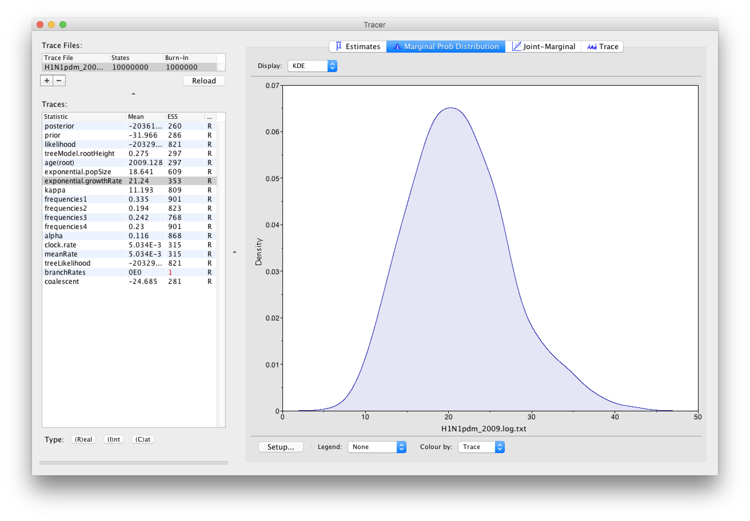
As you can see the posterior probability density is roughly bell-shaped. The default is to show the kernel density estimate (KDE) which is smoothed probability density fitted to the data. Switch the Display: option at the top to Histogram to see the unsmoothed frequency plot. There is still a lot of noise here but it is a good estimate of the distribution.
age(root) statistic provides an estimate of the time of the most recent common ancestor of the entire tree. In this case it may be a reasonable estimate of the start of the epidemic, when the virus jumped from pigs into humans. What is the mean estimate and 95% HPDs for the date of the MRCA?You can visualize the growth estimate using the Demographic Reconstruction... option in the Analysis menu. Select this option and set up the dialog box that appears like this:
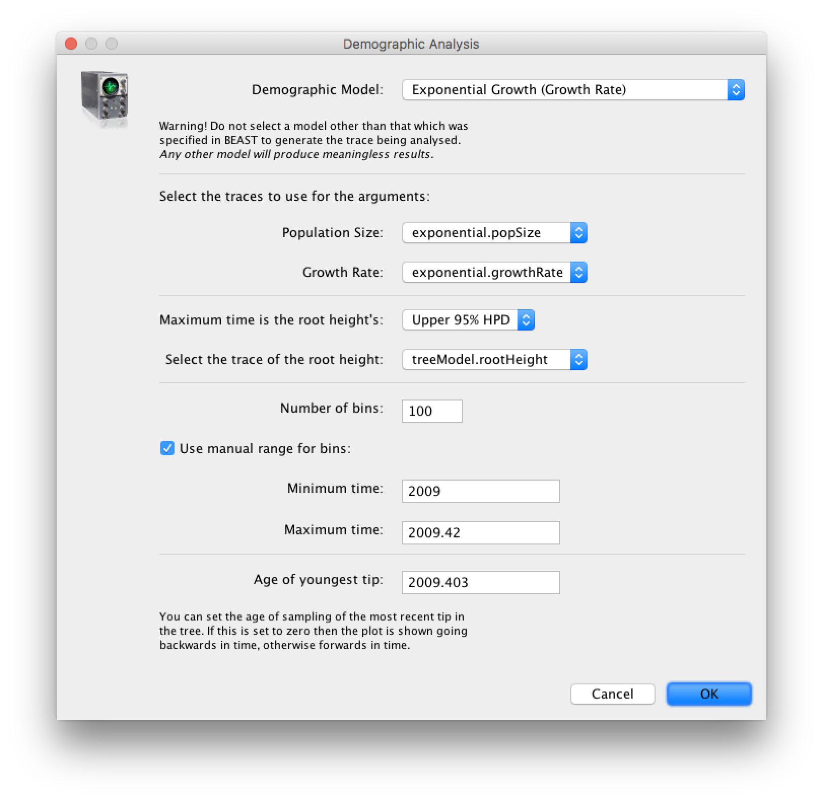
Select Demographic Model: Exponential Growth (Growth Rate) — note, you must select the tree prior you picked in BEAUti, you can’t change this here. Tracer will automatically identify the parameters of the model (exponential.popSize and exponential.growthRate). The option Maximum time is the root height's: pick the Upper 95% HPD. This means it will extend the reconstruction back to the extent of the root age credible interval. Set the Age of youngest tip: to 2009.403 (the date of the most recently sampled virus). You can also Use manual range for bins: to make the time-scale a bit cleaner — choose 2009.0 to 2009.42. Then press OK and this window will appear:
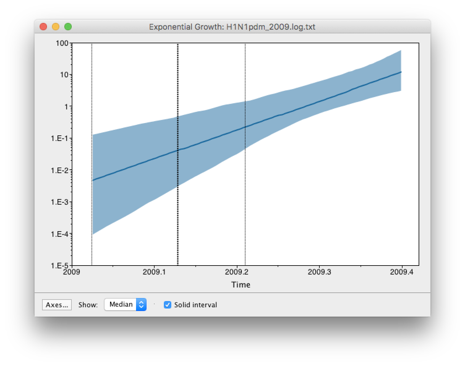
This shows the exponential growth line for the median growth rate and the 95% HPD intervals for this growth as a solid area. It is on a log scale so is a straight line. You can play with the axis settings using the Setup... button. The dotted vertical lines represent the 95% HPD for the date of the root of the tree.
Summarizing the trees
We have seen how we can diagnose our MCMC run using Tracer and produce estimates of the marginal posterior distributions of parameters of our model. Next we can use the TreeAnnotator tool that is provided as part of the BEAST package to summarize the information contained within our sampled trees.
TreeAnnotator takes a single ‘target’ tree and annotates it with the summarized information from the entire sample of trees. The summarized information includes the average node ages (along with the HPD intervals), the posterior support and the average rate of evolution on each branch (for relaxed clock models where this can vary). The program calculates these values for each node or clade observed in the specified ‘target’ tree.
Use a Burnin (as states): of 1,000,000. This is 10% of the chain and we confirmed that this was adequate in Tracer, above. Use the defaults for the rest of the options — Posterior probability limit: 0, Target tree type: Maximum clade credibility tree, and Node heights: Median.
Use the Choose File... button to select an input trees file, H1N1pdm_2009.log.
Select a name for the output tree file (e.g., H1N1pdm_2009.MCC.tre).
Once you have selected all the options, above, press the Run button. TreeAnnotator will analyse the input tree file and write the summary tree to the file you specified. This tree is in standard NEXUS tree file format so may be loaded into any tree drawing package that supports this. However, it also contains additional information that can only be displayed using the PearTree program.
Viewing the annotated tree
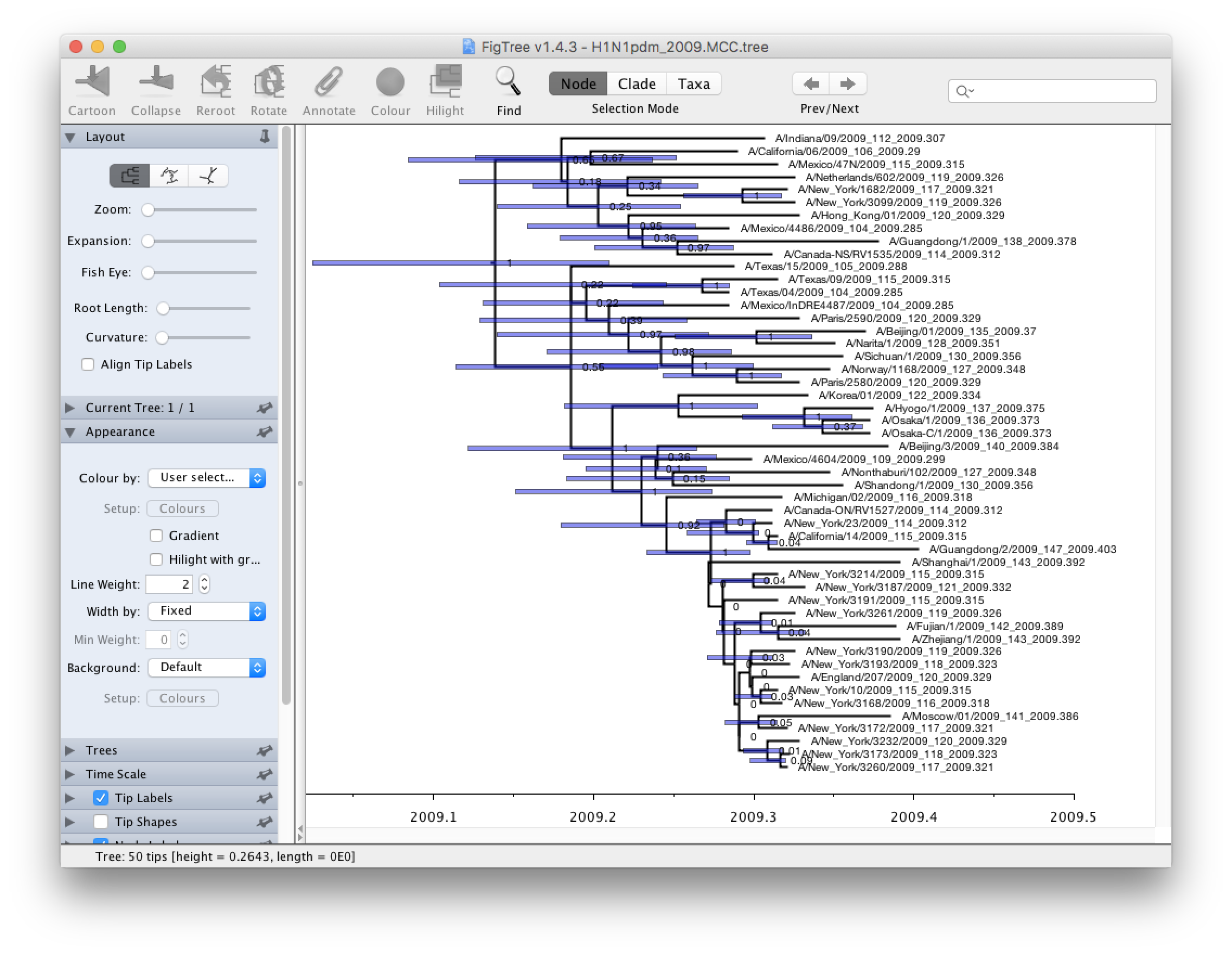
Run PearTree now and select the Open... command from the File menu. Select the tree file you created using TreeAnnotator in the previous section. The tree will be displayed in the PearTree window. On the left hand side of the window are the options and settings which control how the tree is displayed. In this case we want to display the posterior probabilities of each of the clades present in the tree and estimates of the age of each node. In order to do this you need to change some of the settings.
First, re-order the node order by Increasing Node Order under the Tree menu. Switch on Branch Labels in the control panel on the left and open its section by clicking on the arrow on the left. Now select posterior under the Display: option. Reduce Sig. Digits to 2.
We now want to display bars on the tree to represent the estimated uncertainty in the date for each node. TreeAnnotator will have placed this information in the tree file in the shape of the 95% highest posterior density (HPD) credible intervals. Switch on Node Bars in the control panel and open this section; select height_95%_HPD to display the 95% HPDs of the node heights.
We can also plot a time scale axis for this evolutionary history. Switch on Scale Axis (and switch off Scale bar) and select Reverse Axis in the Scale Axis options (you can also increase the font size a bit). For appropriate scaling, open the Time Scale section of the control panel, set the Offset: to 2009.403 (the date of our most recently sampled virus).
Finally, open the Appearance panel and alter the Line Weight to draw the tree with thicker lines. The resulting tree will look like this:
None of the options actually alter the tree’s topology or branch lengths in anyway so feel free to explore the options and settings. You can also save the tree and this will save most of your settings so that when you load it into PearTree again it will be displayed almost exactly as you selected. The tree can also be exported to a graphics file (pdf, eps, etc.).
References
- Smith GJD, Vijaykrishna D, Bahl J, Lycett SJ, Worobey M, Pybus OG, Ma SK, Cheung CL, Raghwani J, Bhatt S, Peiris JSM, Guan Y & Rambaut A (2009) Origins and evolutionary genomics of the 2009 swine-origin H1N1 influenza A epidemic. Nature 459, 1122-1125.
Help and documentation
The BEAST website: http://beast.community
Tutorials: http://beast.community/tutorials
Frequently asked questions: http://beast.community/faq