Setting up Hierarchical Phylogenetic Models (HPMs)
To set up HPM models using this tutorial, you only need to download the BEAST software package in a format that is compatible with your computer system (all three are available for Mac OS X, Windows and Linux/UNIX operating systems):
HPM across Different Partitions within a Species
This first part of the HPM tutorial describes how to set up a BEAST analysis with a hierarchical phylogenetic model (HPM) on substitution model parameters within a single species.
The Influenza B data set used here consists of multiple genes for the same viral sequences; we will focus here on 3 genes: hemagglutinin (HA), neuraminidase (NA) and RNA polymerase subunit (PA).
Start BEAUti, select all the nexus files and drag them into the Partitions panel (or import them using File - Import Data …):
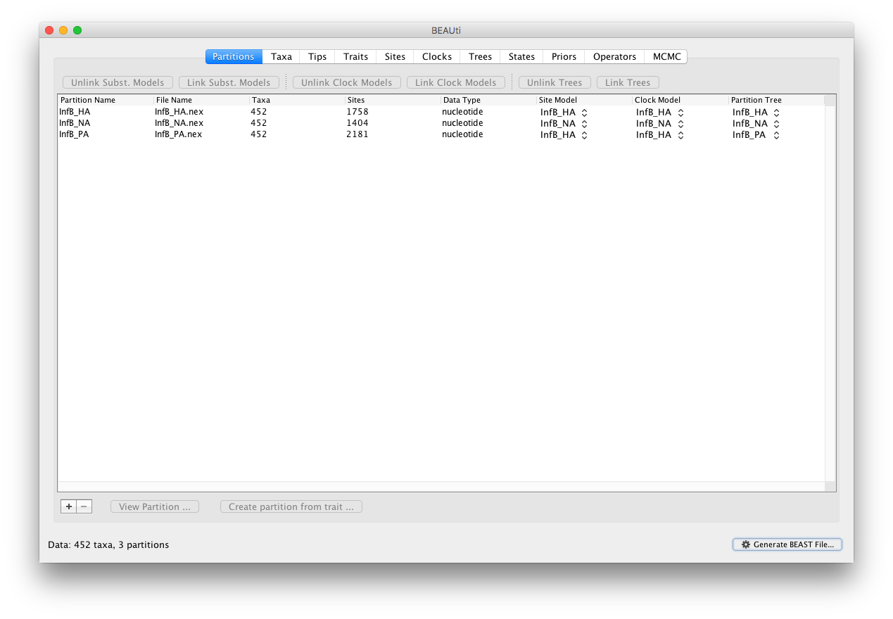
Select all partitions, and click on ‘Unlink Subst. Models’ to allow each lineage to evolve according to different substitution parameters (check that the Site Model has changed and become specific to each partition). Given that these partitions constitute different genes from the same species, we (typically) do not unlink the clock models.
In the Tips panel, be sure to parse the sampling dates from the taxon labels.
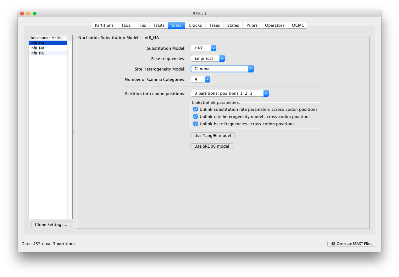
In the Sites panel, keep the default HKY model, but set the ‘Base Frequencies’ to ‘Empirical’ and ‘Site heterogeneity Model’ to ‘Gamma’ for the top partition (i.e. the first one in the list: InfB_HA). Additionally, we’ll partition each gene into 3 codon positions which will generate a total of 9 sequence data partitions:
For this tutorial, we will not alter the settings for the clock model and the coalescent model. In the ‘Priors’ panel, we will specify the hierarchical priors for the substitution model parameters. We can achieve this by cmd-selecting (or ctrl-selecting in Windows for example) all the equivalent parameters across the partitions and using the ‘Link parameters into a hierarchical model’ button at the bottom of the window. First select the kappa parameters in the first codon positions, and select ‘Link parameters into a hierarchical model’. In the new Phylogenetic Hierarchical Model Setup window, enter a Unique Name (e.g. CP1.kappa), set the Normal Hyperprior Stdev to 5.0 and the Gamma Hyperprior Shape and Scale to 0.01 and 100.0 respectively and click OK:
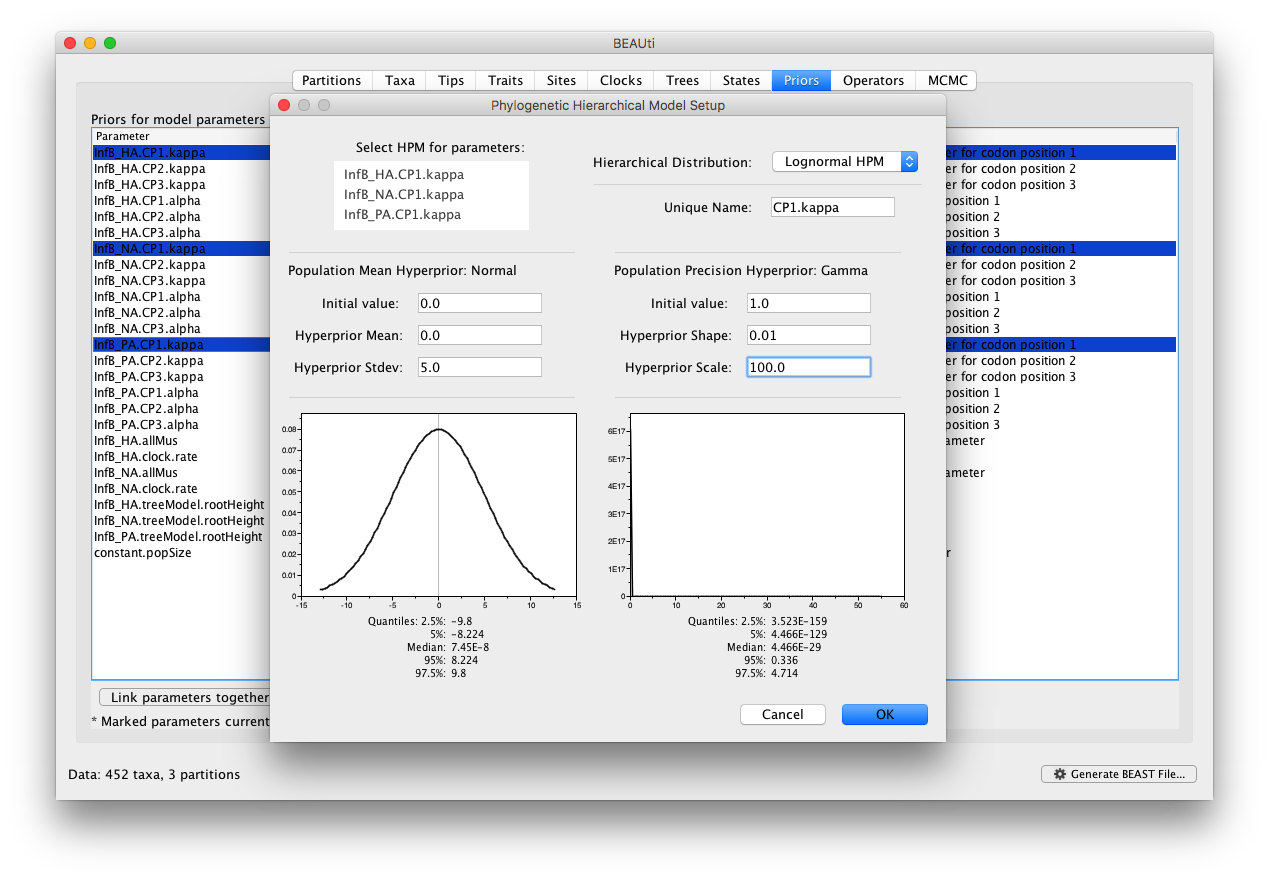
Similarly, we can create HPMs for the kappa parameters at the second codon positions (e.g. CP2.kappa) and at the third codon positions (e.g. CP3.kappa). The alpha parameters, describing among-site rate heterogeneity at each codon position, can also be equipped with an HPM (e.g. CP1.alpha, CP2.alpha and CP3.alpha). In total, we end up with 6 HPMs, equal to the number of codon positions times (3) the different types of parameters across the partitions (2, i.e. kappa and alpha).
HPM across Different Bat Species
This part of the HPM tutorial describes how to set up an BEAST analysis with a hierarchical phylogenetic model (HPM) aimed at identifying the factors responsible for evolutionary rate variation in bat rabies viruses (RABV) based on a data set previously analysed by Streicker et al. (2012). Bat rabies viruses in the Americas have established host-associated lineages through sequential host jumping followed by successful transmission in the new bat species (see Streicker et al., 2010). This provides a rare occasion to test the impact of host factors (physiological, environmental or ecological) on virus evolutionary rates. We will here set up an xml using BEAUti that specifies hierarchical prior distributions for the clock rates and substitution model parameters.
Separate alignments in fasta format are available for each host-associated lineage and can be downloaded below.
Start BEAUti, select all the fasta files and drag them into the Partitions panel:
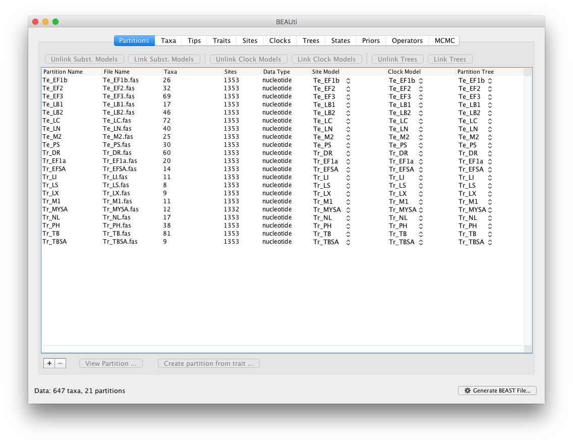
Select all partitions, and click on ‘Unlink Subst. Models’ to allow each lineage to evolve according to different substitution parameters (check that the Site Model has changed and become specific to each partition). Also select ‘Unlink Clock Models’ to allow each lineage to evolve under different rates of evolution (check that the Clock Model has become specific to each partition).
In the Tips panel, be sure to parse the sampling dates from the taxon labels (use ‘Parse Dates’. set the Order to ‘last’ and click OK.).
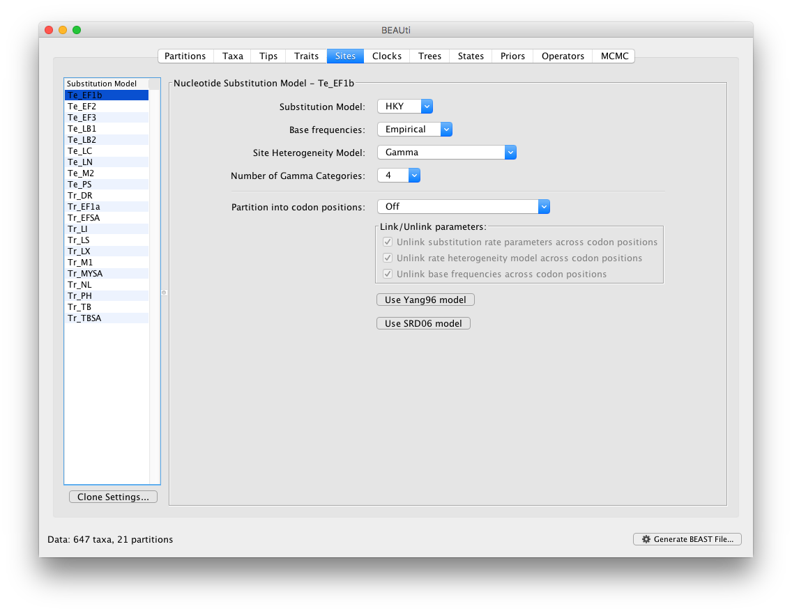
In the Sites panel, keep the default HKY model, but set the ‘Base Frequencies’ to ‘Empirical’ and ‘Site heterogeneity Model’ to ‘Gamma’ for the top partition (i.e. the first one in the list: Te_EF1b):
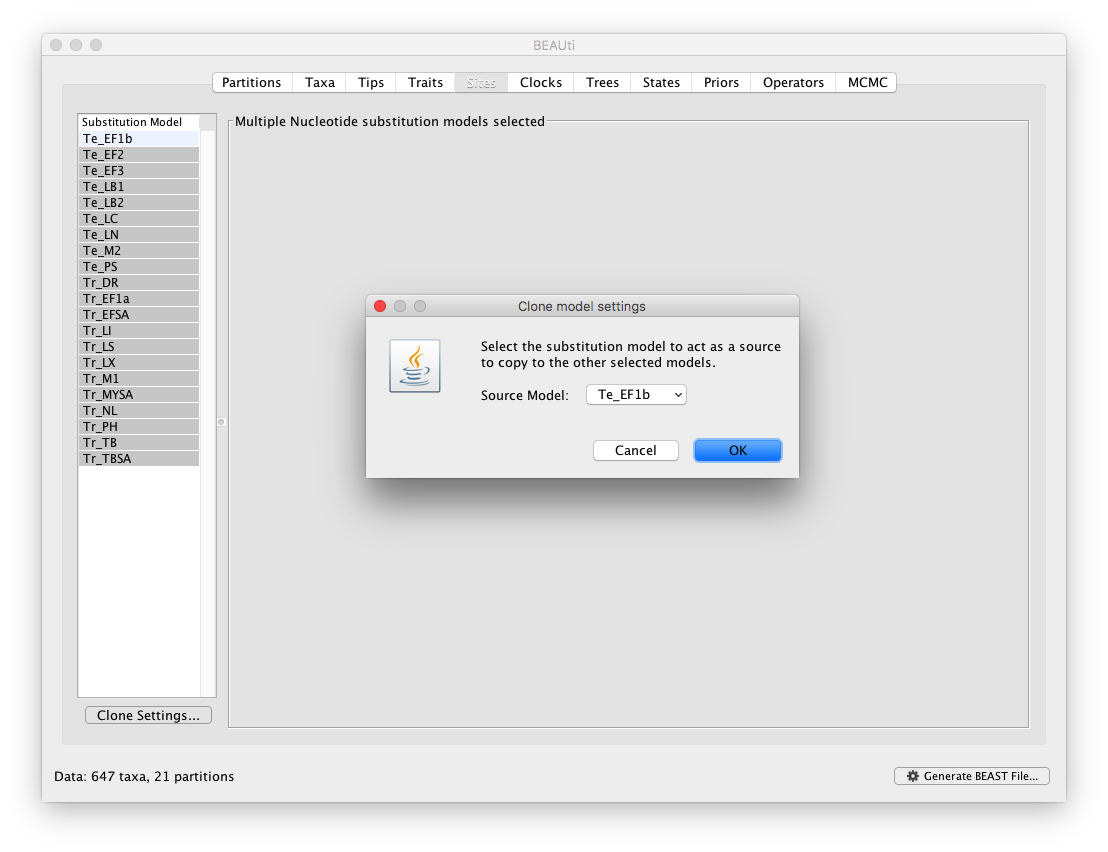
To apply the same settings to all other partitions, select all partitions and click on the ‘Clone Settings’ button and keep the default ‘Te_EF1b’ partition as source model for the cloning:
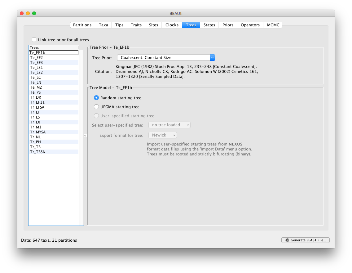
Keep the default ‘Strict Clock’ model in the Clocks panel for all the partitions. In the ‘Trees’ panel, make sure to unlink the tree prior (in the top left of the panel), and keep the default constant population size model as a simple tree prior.
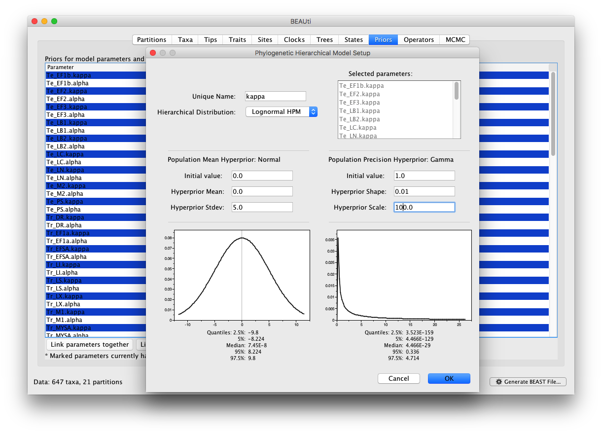
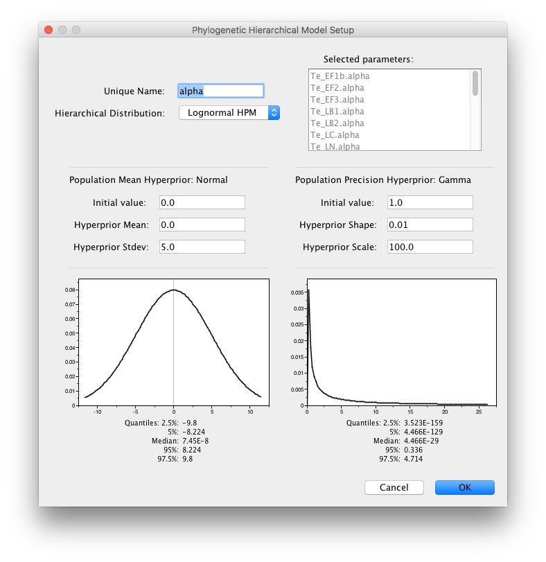
In the ‘Priors’ panel, we will specify the hierarchical priors for the substitution model parameters and the clock rates. We can achieve this by cmd-selecting (or ctrl-selecting in Windows for example) all the equivalent parameters across the partitions and using the ‘Link parameters into a hierarchical model’ button at the bottom of the window. First cmd-select all kappa parameters, and select ‘Link parameters into a hierarchical model’. In the new Phylogenetic Hierarchical Model Setup window, enter a Unique Name (e.g. kappa), set the Normal Hyperprior Stdev to 5.0 and the Gamma Hyperprior Shape and Scale to 0.01 and 100.0 respectively and click OK:
This operation can be repeated for the ‘alpha’ parameters with the same hyperprior settings and ‘alpha’ as Unique Name.
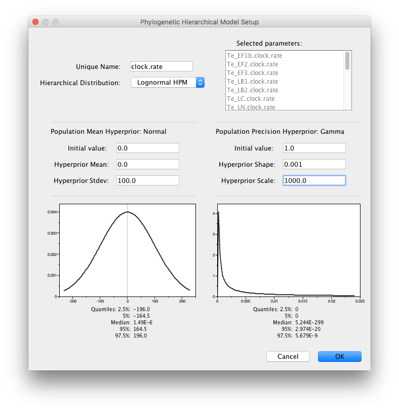
A similar HPM can be created for the clock.rate parameters and the population sizes of the coalescent models. To this end, shift select the first and the last clock.rate to select all clock.rate parameters and click ‘Link parameters into a hierarchical model’. Provide clock.rate as unique name and set the Normal Hyperprior Stdev to 100.0 and the Gamma Hyperprior Shape and Scale to 0.001 and 1000.0 respectively and click OK:
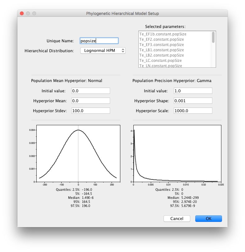
Finally, specify an HPM for the pop sizes by shift-selecting them and setting the Normal Hyperprior Stdev to 100.0 and the Gamma Hyperprior Shape and Scale to 0.001 and 1000.0.
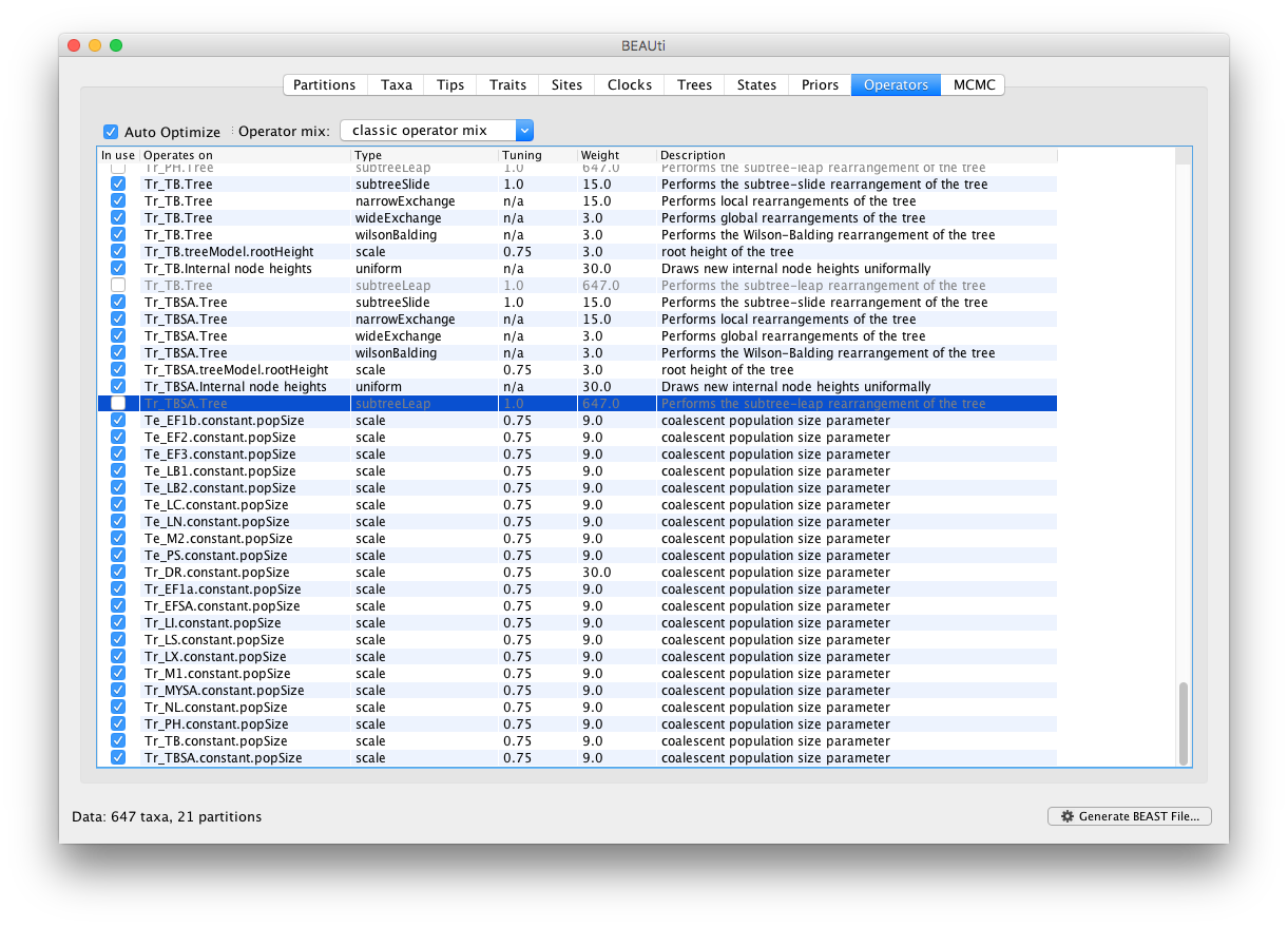
In our experience with this data, efficient mixing of the pop sizes is difficult to obtain. To address this, we will increase the weight on the scale operators for the pop sizes from 3 to 9 in Operators panel. The mixing is particularly problematic for Tr_DR and hence we set the weight of this operator to 30.
In the mcmc panel, set the chain frequency to 250,000,000 and the logging frequency to 250,000 and provide ‘BatRabies_HPM’ as File stem name:
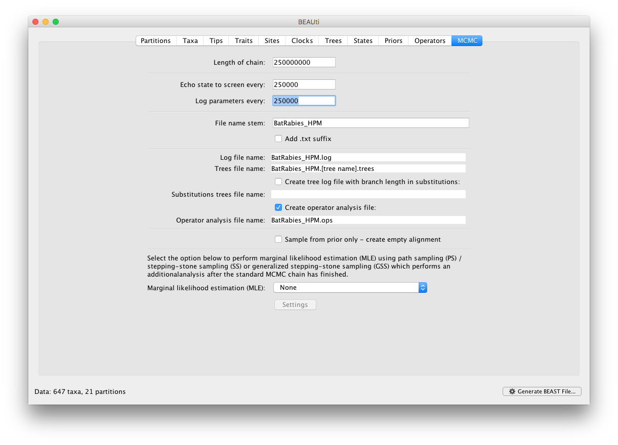
We run a relatively chain for this analysis because we need to operate on a large set of parameters (each of the 21 alignments/partitions is associated with its own phylogeny, substitution model and clock rate). Check that the xml file runs in BEAST, but there is no real need to run this to completion.
We can also examine whether there is a difference in substitution rates for rabies viruses in bats in temperate climate (with a ‘Te_’ prefix) compared to viral lineages in bats in subtropical and tropical climates (with a ‘Tr_’ prefix). To do this, we can put independent hierarchical priors over all clock rates for partitions with the ‘Te_’ prefix and over all clock rates for partitions with the ‘Tr_’ prefix in Priors panel. A long run is available to examine the results; in this case the hierarchical means in the log files are ‘Te_clock.rate.mean’ and ‘Tr_clock.rate.mean’ (they are in log space).
Is there a difference in overall rate, and if so, which viruses tend to evolve faster?
References
Streicker D. G., Turmelle A. S., Vonhof M. J., Kuzmin I. V., McCracken G. F., Rupprecht C. E. (2010) Host phylogeny constrains cross-species emergence and establishment of rabies virus in bats. Science 329:676-679.
Streicker D. G., Altizer S. M., Velasco-Villa A. and Rupprecht C. E. (2012) Variable evolutionary routes to host establishment across repeated rabies virus host shifts among bats. Proc. Natl. Acad. Sci. USA 109(48): 19715-19720.