Time Dependent Rates | BEAST Documentation

Setting up a time-dependent rate (TDR) model in BEAST.

Time Dependent Rate Model Tutorial

The tutorial combines the concept of epoch modelling, discussed in the ‘Epoch model’ tutorial, and a generalized linear model formulation for the epoch parameters.

As example dataset, we use the foamy virus (FV) dataset analyzed by Aiewsakun and Katzourakis (2015) to show the presence of time dependent rates. The input file for this tutorial, TDRP_foamy.fas, can be downloaded here

Note that in this dataset, we consider a time scale in millions of years (My). We use this data set to demonstrate how to apply the time dependent rate (TDR) clock model described in Membrebe et al. (2019). We first create an xml using BEAuti which will serve as the basis for further editing in order to set up the epoch-TDR model.

Generating an XML File

The first thing that we need to do is to upload the sequences in BEAUti and generate an XML file. Upload the dataset in the Partitions tab. The TDR model requires internal node calibrations, preferrably distributed across the time-scale of the evolutionary history. Because of the history of FV-host co-speciation, we can calibrate most nodes in the FV tree using estimates of host divergence dates. To specify such calibrations, we first need to define taxon sets for the relevant nodes as follows in the Taxa panel and enforce them to be monophyletic:

Taxon Set	Included Taxa
node1	PFV,SFVcpz
node2	PFV,SFVcpz,SFVbnb
node3	PFV,SFVcpz,SFVbnb,SFVgor
node4	SFVmac,SFVagm
node5	PFV,SFVcpz,SFVbnb,SFVgor,SFVora
node6	PFV,SFVcpz,SFVbnb,SFVgor,SFVora,SFVmac,SFVagm
node7	PFV,SFVcpz,SFVbnb,SFVgor,SFVora,SFVmac,SFVagm,SFVsqu,SFVmar,SFVspm
node8	PFV,SFVcpz,SFVbnb,SFVgor,SFVora,SFVmac,SFVagm,SFVsqu,SFVmar,SFVspm,PSFVgal
node9	BFV,EFV
node10	BFV,EFV,FFV

In the Sites panel, we select the general time-reversible (GTR) substitution model for a single nucleotide partition, keep the base frequencies as ‘Estimated’ and select ‘Gamma’ distributed rate heterogeneity among sites. We keep the Clock model as ‘Strict clock’ for now in the Clocks panel. In the Trees panel, we select a Yule speciation model. In the Priors panel, we would be able to set up all the calibration distributions for the nodes we have set as taxa sets. However, we will do this when editing the xml and keep all priors to their defaults for now.

Finally, we generate the XML file which should look like this.

Specifying the Time Dependent Rate Clock Model

The next step is to edit the XML file that we have created in the previous section to incorporate an epoch-TDR model. To do this, look for the block where the clock model and its associated rate statistic has been defined and delete this. We will replace this with our TDR clock model.

	<!-- The strict clock (Uniform rates across branches)                        -->
	<strictClockBranchRates id="branchRates">
		<rate>
			<parameter id="clock.rate" value="1.0"/>
		</rate>
	</strictClockBranchRates>
	
	<rateStatistic id="meanRate" name="meanRate" mode="mean" internal="true" external="true">
		<treeModel idref="treeModel"/>
		<strictClockBranchRates idref="branchRates"/>
	</rateStatistic>

To allow rates to vary over time, we will set up an epoch structure that specifies a different rate parameter for each epoch interval and then model a specific relationshop between these epoch rates. Membrebe et al. (2019) explore to different epoch structures that cover a time period beyond the expected depth of the phylogeny. For this tutorial, we follow the exponential epoch structure and create the boundaries of the epochs as \(0 < 10^{-5} < 10^{-5} < ... < 10^{2} < \infty\) My. Hence, the first epoch is bounded between 0 and 10 years into the past. The alternative uniform epoch structure set up in Membrebe et al. (2019) used the following boundaries: \(0 < 10 < 20 < ... < 90 < \infty\) My.

Next, we must compute the values of the time-covariates for the rates in our TDR clock model, which has the form:

\[\log r_m = \beta_0 + \beta_1 \log t_m\]

In this model, we parameterize each epoch rate (\(r_m\)) as a log-linear function of time. The parameter \(\beta_0\) represents the log rate at log(time) = 0, while \(\beta_1\) quantifies the time-dependent effect. For the time-covariate \(t_m\), we take the midpoint of epoch \(m\) (\(m=1,...,M\) epochs). However, we must put the natural logarithm of this value in our XML file. So, for the first epoch, this value is log(5)=-12.2060726455. Because the last epoch extends to \(\infty\), we assume in practice an alternative time for its midpoint that extends the time series of the preceding boundaries in order to compute a finite last midpoint time. That is, for the last epoch, the time-covariate value is log(550)=6.3099182782

Where we deleted the strict clock model, paste the following blocks that specify the generalized linear model (GLM) for all the rates (‘all.rates’) on a log-scale through a ‘designMatrix’ and a ‘matrixVectorProductParameter’:

    <designMatrix id="epochDesignMatrix">
        <parameter id="designMatrix.offset" value="1 1 1 1 1 1 1 1 1"/> 
        <parameter id="designMatrix.time"   value="-12.2060726455 -9.8081773727 -7.5055922797 -5.2030071867 -2.9004220937 -0.5978370008 1.7047480922 4.0073331852 6.3099182782"/>
    </designMatrix>

	<matrixVectorProductParameter id="all.rates">
		<matrix>
			<designMatrix idref="epochDesignMatrix"/>
		</matrix>
		<vector>
			<parameter id="rate.coefficients" value="-4 -0.05"/>
	    </vector>
	</matrixVectorProductParameter>

In this GLM specification, the values of the ‘designMatrix.time’ parameter are the natural logarithms of the midpoints of each epoch. Note that the dimension of GLM specification in this case corresponds to nine rates and hence nine epochs. This epoch-covariate specification will need to be adjusted for each specific data set that needs to be analyzed. The values of the rate.coefficients parameter, \(\beta_0\) and \(\beta_1\) respectively, provide starting values for the GLM parameters.

In the epoch specification that will follow, we will need to associate each epoch interval with a specific rate on a natural scale. For this purpose, we create a transformed parameter for each epoch rate that pulls a single rate out of the ‘all.rates’ parameter vector using a ‘maskedParameter’. The inverse=”true” argument transforms the log rate back to the natural scale. The transformedParameter block for the first epoch rate should be pasted after the ‘matrixVectorProductParameter’ block and should look like the following:

	<transformedParameter id="epoch.rate01" inverse="true">
		<transform type="log"/>
		<maskedParameter signalDependents="false">
			<parameter idref="all.rates"/>
			<mask>
				<parameter value="1 0 0 0 0 0 0 0 0"/>  
			</mask>
		</maskedParameter>
	</transformedParameter>

In this case, the ‘maskedParameter’ pulls out the first rate from the ‘all.rates’ parameter vector, which is why we define the ‘transformedParameter’ as epoch.rate01. Create a transformedParameter block for each epoch, while adjusting its ‘id’ and the value of the masking parameter value. That is, the last block should look like the following:

	<transformedParameter id="epoch.rate09" inverse="true">
		<transform type="log"/>
		<maskedParameter signalDependents="false">
			<parameter idref="all.rates"/>
			<mask>
				<parameter value="0 0 0 0 0 0 0 0 1"/>  
			</mask>
		</maskedParameter>
	</transformedParameter>

Next, we need to create the actual epoch structure for the rates by pasting the following ‘rateEpochBranchRates’ after the ‘transformedParameter’ blocks:

	<rateEpochBranchRates id="epochRates">
		<epoch transitionTime="0.00001">
			<parameter idref="epoch.rate01"/>
		</epoch>
		<epoch transitionTime="0.0001">
			<parameter idref="epoch.rate02"/>
		</epoch>
		<epoch transitionTime="0.001">
			<parameter idref="epoch.rate03"/>
		</epoch>
		<epoch transitionTime="0.01">
			<parameter idref="epoch.rate04"/>
		</epoch>
		<epoch transitionTime="0.1">
			<parameter idref="epoch.rate05"/>
		</epoch>
		<epoch transitionTime="1">
			<parameter idref="epoch.rate06"/>
		</epoch>
		<epoch transitionTime="10">
			<parameter idref="epoch.rate07"/>
		</epoch>
		<epoch transitionTime="100">
			<parameter idref="epoch.rate08"/>
		</epoch>
		<rate>
			<parameter idref="epoch.rate09"/>
		</rate>
		<rootHeight>
			<parameter idref="treeModel.rootHeight"/>
		</rootHeight>
	</rateEpochBranchRates>

The ‘rateEpochBranchRates’ creates the epoch intervals (through transition times) and associates each epoch interval with an individual rate. In this case, the rate referred to as ‘epoch.rate01’ is associated with the interval from time 0 to 0.00001 My, the rate ‘epoch.rate02’ is the rate from time 0.00001 My to 0.0001 My, and so on.

In addition, we can create a compound parameter which compiles all the epoch rates (on a natural scale). To this purpose, paste the following after the ‘rateEpochBranchRates’ block:

	<compoundParameter id="epoch.rates">
		<parameter idref="epoch.rate01"/>
		<parameter idref="epoch.rate02"/>
		<parameter idref="epoch.rate03"/>
		<parameter idref="epoch.rate04"/>
		<parameter idref="epoch.rate05"/>
		<parameter idref="epoch.rate06"/>
		<parameter idref="epoch.rate07"/>
		<parameter idref="epoch.rate08"/>
		<parameter idref="epoch.rate09"/>
	</compoundParameter>

Finally, we need to instruct BEAST to use the values of the epochRates and not the strict clock branch rates, which was in the original file we generated from BEAUti, when computing the likelihood. To this purpose, we reference our TDR model in the ‘treeDataLikelihood’ block instead of the branchRates as follows:

	<treeDataLikelihood id="treeLikelihood" useAmbiguities="false">
		<partition>
			<patterns idref="patterns"/>
			<siteModel idref="siteModel"/>
		</partition>
		<treeModel idref="treeModel"/>
		<rateEpochBranchRates idref="epochRates"/>
	</treeDataLikelihood>

In the operators block, we define a random walk operator for the rate coefficients. Paste this XML block within the operators block:

	<randomWalkOperator windowSize="0.01" weight="5"  autoOptimize="true">
		<parameter idref="rate.coefficients"/>
	</randomWalkOperator> 

In the prior block (part of the mcmc block), delete the ‘strictClockBranchRates’ line, and replace this with ‘rateEpochBranchRates’:

	    <rateEpochBranchRates idref="epochRates"/>

In addition, we will also add the calibrations to the prior block. These calibrations are important in our analysis as these are the data that BEAST uses to inform our TDR model. These ten internal node calibrations and one MRCA calibration were presented in the study of Aiewsakun and Katzourakis (2015). Paste the following codes in the prior block:

    <normalPrior mean="0.96" stdev="0.133">
        <statistic idref="tmrca(node1)"/>
    </normalPrior>

    <normalPrior mean="2.17" stdev="0.531">
        <statistic idref="tmrca(node2)"/>
    </normalPrior>

    <normalPrior mean="8.3" stdev="0.903">
        <statistic idref="tmrca(node3)"/>
    </normalPrior>

    <normalPrior mean="11.50" stdev="1.199">
        <statistic idref="tmrca(node4)"/>
    </normalPrior>

    <normalPrior mean="16.52" stdev="1.610">
        <statistic idref="tmrca(node5)"/>
    </normalPrior>

    <normalPrior mean="31.56" stdev="3.225">
        <statistic idref="tmrca(node6)"/>
    </normalPrior>

    <normalPrior mean="43.47" stdev="2.51">
        <statistic idref="tmrca(node7)"/>
    </normalPrior>

    <normalPrior mean="87.18" stdev="5.847">
        <statistic idref="tmrca(node8)"/>
    </normalPrior>

    <normalPrior mean="87.3" stdev="1.02">
        <statistic idref="tmrca(node9)"/>
    </normalPrior>

    <normalPrior mean="88.7" stdev="1.02">
        <statistic idref="tmrca(node10)"/>
    </normalPrior>

    <normalPrior mean="98.9" stdev="1.378">
        <parameter idref="treeModel.rootHeight"/>
    </normalPrior>

We also need to specify a prior over our rate coefficients in the priors block. In this case, we specify a multivariate normal prior with the parameterization used in Membrebe et al. (2019). Paste the following lines in the mcmc block, within the prior section:

    <multivariateNormalPrior id="rate.prior.effects">
        <data>
            <parameter idref="rate.coefficients"/>
        </data>
        <meanParameter>
            <parameter value="0 0"/>
        </meanParameter>
        <precisionParameter>
            <matrixParameter>
                <parameter value="0.001 0"/>
                <parameter value="0 0.5"/>
            </matrixParameter>
        </precisionParameter>
    </multivariateNormalPrior>

In the screenLog block, you can add a column to monitor the rate coefficients:

    <column sf="6" width="12">
        <parameter idref="rate.coefficients"/>
    </column>

In order to log the coefficients of our TDR model and the value of the individual epoch rates to file, add the following lines to the fileLog block:

        <parameter idref="rate.coefficients"/>
        <compoundParameter idref="epoch.rates"/>

Delete these lines in the fileLog block as BEAST would not compute them anymore:

        <strictClockBranchRates idref="branchRates"/>
        <parameter idref="clock.rate"/>
        <rateStatistic idref="meanRate"/>

Finally, in the treeFileLog block, delete the line with the ‘branchRates ‘and replace this with the ‘epochRates’:

        <rateEpochBranchRates idref="epochRates"/>

We have now completed the XML editing and we can analyze this using BEAST. The final XML file should look like this

Running BEAST

Run the XML file in BEAST. We recommend to use BEAGLE with BEAST to increase the performance in terms of computation time. The installation and setup of the BEAGLE library on various platforms is covered on this website.

We can run BEAST using either the GUI interface or using the command line.

Analyzing the Output

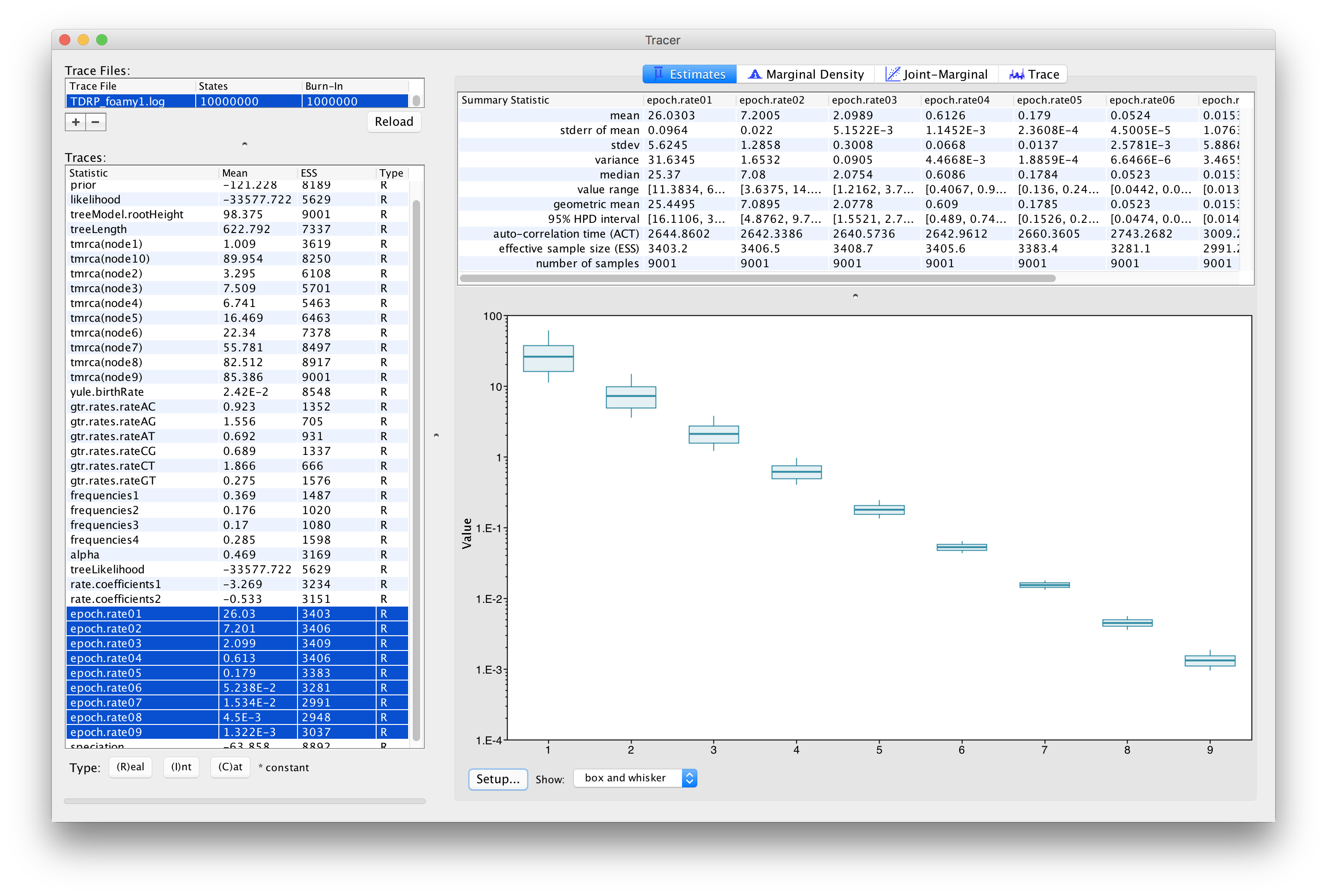
Once the analysis has been finished, you load the log file in Tracer to diagnize and summarize the MCMC run.

In our analysis, we obtained an estimate that indicates a strong TDR effect (\(\beta_1 = -0.533 [-0.594, -0.475]\)). In fact, this can be seen in Figure 1, which is a plot that shows the different epoch rate estimates in a log-time scale. In comparison to a previous estimate (Schweizer et al., 1999) for the short-term FV rate of \(3.75\times 10^{-4}\) substitutions/site/year (s/s/yr), we estimate a lower rate close to the present (2.60 [95\% highest posterior density interval: 1.61–3.73] \(10^{-5}\) s/s/yr at \(t_m = 5\) years). At the same time, the epoch models infer very slow evolutionary rates close to the root of the phylogeny (1.32 [95\% highest posterior density interval: 1.11–1.54] \(10^{-9}\) s/s/yr at 99 My)

References

Aiewsakun P, Katzourakis A. 2015. Time dependency of foamy virus evolutionary rate estimates. BMC Evol Biol. 15:119.

Ho SY, Duchene S, Molak M, Shapiro B. 2015. Time-dependent estimates of molecular evolutionary rates: evidence and causes. Mol Ecol. 24(24):6007–6012.

Membrebe, J. V., Suchard, M. A., Rambaut, A., Baele, G., Lemey, P. (2019) Bayesian inference of evolutionary histories under time-dependent substitution rates. Mol. Biol. Evol. 36(8):1793-1803.

Tags: