Introduction
Spatiotemporal bias in genome sequence sampling can severely confound phylogeographic inference based on discrete trait ancestral reconstruction. This has impeded our ability to accurately track the emergence and spread of SARS-CoV-2, which is the virus responsible for the COVID-19 pandemic. Along with the unprecedented accumulation of genomic sequences from across the world comes a vast collection of metadata on individual patients, such as - in some cases - details on their recent movements such as travel history prior to having developed any symptoms. This information can be exploited, as we will show here, in order to yield more realistic reconstructions of virus spread, particularly when travelers from undersampled locations are included to mitigate sampling bias.
Example dataset
The small example dataset here consists of 9 SARS-CoV-2 sequences, sampled from 3 different locations: Australia (4), Italy (3) and Wuhan (2).
We refer to the pre-print (Lemey et al., 2020) for a large(r) real-life analysis from the COVID-19 pandemic. All analyses have been performed using a custom build of BEAST 1.10.5 (see below for the download link; Suchard et al., 2018). Incorporating an individual’s travel history to the phylogeographic analysis requires manual XML editing in order to specify the different model components.
Discrete phylogeographic inference
Discrete (trait) phylogeographic inference (Lemey et al., 2009) attempts to reconstruct an ancestral location-transition history along a phylogeny based on the discrete states associated with the sampled sequences. In this tutorial, we will consider three different ways of performing Bayesian phylogeographic inference. These approaches differ in the way that the sampling locations and travel history are being used/accommodated. The remaining model specifications are however identical: an exponentially growing population size, a single substitution model across the entire alignment (HKY+G) and a strict molecular clock model. The default prior on the growth rate of the coalescent model has been replaced by the following:
    <laplacePrior mean="0.0" scale="100.0">
        <parameter idref="exponential.growthRate"/>
    </laplacePrior>
Note that in order to visualize the complete transition history throughout a phylogeny, we are required to reconstruct the complete state change history of the location trait along the trees.
This can be easily set up in BEAUti by following the phylogeographic diffusion in discrete space tutorial.
By default, BEAUti will create a separate logTree output file that only includes the Markov jump histories.
To visualize these Markov jump trajectories, we must add the state node annotations into this file as follows:
    <logTree logEvery="10000" nexusFormat="true" fileName="9seqs_sample.loc.history.trees" sortTranslationTable="true">
        <treeModel idref="treeModel"/>
        <!-- Location node annotations -->
        <trait name="loc.states" tag="loc">
            <ancestralTreeLikelihood idref="loc.treeLikelihood"/>
        </trait>
        <!-- Markov Jump histories -->
        <markovJumpsTreeLikelihood idref="loc.treeLikelihood"/>
    </logTree>
In the following 3 subsections, we show how to specify these 3 different discrete phylogeographic approaches and discuss how they impact inference results.
Using only location of sampling
When the sampling location of a sequence is available, the tip state for that sequence in the phylogeny can be set to this location. This corresponds to the classic discrete phylogeographic inference scenario (Lemey et al., 2009), and is typically used in the absence of travel (history) information. As a result, only the 3 sampling locations are part of the location data type in the XML specification for this dataset:
    <generalDataType id="loc.dataType">
        <!-- Number Of States = 3 -->
        <state code="Australia"/>
        <state code="Italy"/>
        <state code="Wuhan"/>
    </generalDataType>
Such an analysis can be completely specified using the current version of BEAUti without requiring any manual XML editing. We refer to the following tutorial for more information on how to set up this type of analysis: phylogeographic diffusion in discrete space.
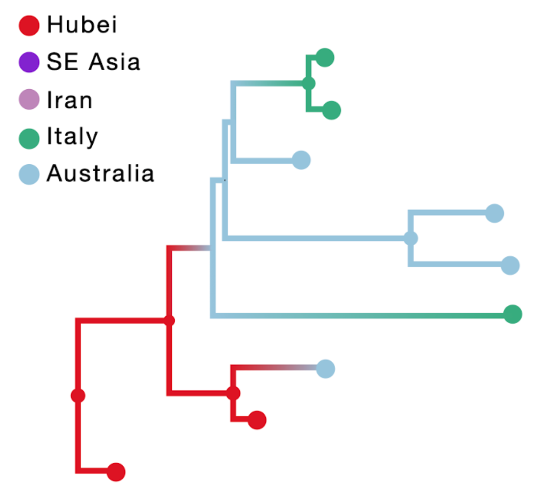
The result of this inference is shown in the figure above; the branch color reflects the modal state estimate at the child node. Using sampling location only results in an unrealistic Australian ancestry and two transitions from Australia to Italy, likely because Australia is represented by the largest number of tips.
Using the location from which an individual travelled
In the previous section, the tip location state for a sequence was set to the location of sampling. However, when information on travel history is available, the tip location state for a sequence can also be set to the location from which the individual travelled (assuming that this was the location from which the infection was acquired). Such an approach constitutes a small variation of standard discrete phylogeographic inference, and we show some of the changes to the provided location information here:
<taxa id="taxa">
    ...
    <taxon id="Australia/VIC01/2020|EPI_ISL_406844|2020-01-25">
        <date value="2020.0655737704917" direction="forwards" units="years"/>
        <attr name="loc">
            Wuhan
            <!-- travel: Wuhan -->
            <!-- sampled: Australia -->
        </attr>
    </taxon>
    ...
    <taxon id="Italy/INMI1-cs/2020|EPI_ISL_410546|2020-01-31">
        <date value="2020.0819672131147" direction="forwards" units="years"/>
        <attr name="loc">
            Wuhan
            <!-- travel: Wuhan -->
            <!-- sampled: Italy -->
        </attr>
    </taxon>
    ...
</taxa>
The XML block above shows some of the changes that were made in the <taxa>...</taxa> block to incorporate information on travel origin location.
As a result of including these additional travel origin locations, the data type that describes the number of locations for this analysis now contains 5 locations:
    <generalDataType id="loc.dataType">
        <!-- Number Of States = 5 -->
        <state code="Australia"/>
        <state code="Italy"/>
        <state code="Iran"/>
        <state code="SEasia"/>
        <state code="Wuhan"/>
    </generalDataType>
Other than replacing the sampling locations for some of the sequences with the locations where these individuals were infected, and augmenting the number of possible locations in the data type accordingly, the rest of the XML file remains unchanged compared to the previous approach.
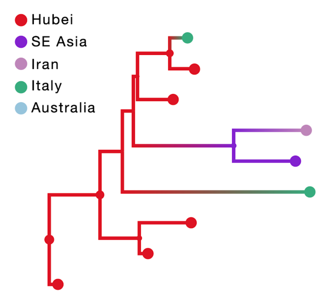
The result of this inference is shown in the figure above; the branch color reflects the modal state estimate at the child node. Using the location of travel origin results in a reconstruction that misses transitions along four tip branches and differs from the reconstruction including travel history for the upper two Italian genomes. Specifically it implies an independent transition from Hubei for the Italian patient that does not have travel history.
Using location of sampling and travel history
Unfortunately, neither of the two previous approaches offers a satisfactory solution. Using only the location of sampling ignores important information about the ancestral location of the sequence, whereas using the travel location together with the collection date represents a data mismatch and ignores the final transitions to the location of sampling. These events are particularly important when the infected traveller then produces a productive transmission chain in the sampling location.
We propose to accommodate travel histories by augmenting the phylogeny with ancestral nodes that are associated with a location state (but not with a known sequence) and hence enforce that ancestral location at a particular, possibly random point in the past of a lineage.
Apart from the standard <taxa>...</taxa> block in the XML file, we need to provide the origin location of each individual’s travel when available.
For our dataset, this additional XML block looks as follows:
<!-- Travel history: defining ancestral node taxa with their discrete trait state -->
    <taxa id="ancestralTaxa">
        <taxon id="Australia/NSW11/2020|EPI_ISL_413597|2020-03-02_ancestor_taxon">
            <attr name="loc">
                Iran
            </attr>
        </taxon>
        <taxon id="Australia/NSW09/2020|EPI_ISL_413595|2020-02-28_ancestor_taxon">
            <attr name="loc">
                SEasia
            </attr>
        </taxon>
        <taxon id="Australia/VIC01/2020|EPI_ISL_406844|2020-01-25_ancestor_taxon">
            <attr name="loc">
                Wuhan
            </attr>
        </taxon>
        <taxon id="Australia/QLD02/2020|EPI_ISL_407896|2020-01-30_ancestor_taxon">
            <attr name="loc">
                Wuhan
            </attr>
        </taxon>
        <taxon id="Italy/INMI1-cs/2020|EPI_ISL_410546|2020-01-31_ancestor_taxon">
            <attr name="loc">
                Wuhan
            </attr>
        </taxon>
    </taxa>
Our augmented dataset is thus specified in a new <taxa> element that contains all sampled and ancestral taxa:
    <taxa id="allTaxa">
        <taxa idref="taxa"/>
        <taxa idref="ancestralTaxa"/>
    </taxa>
The combined collection of discrete locations (i.e. sampling location and origin location of each travelling individual) then make up the 5 possible states of the location data type:
    <generalDataType id="loc.dataType">
        <!-- Number Of States = 5 -->
        <state code="Australia"/>
        <state code="Italy"/>
        <state code="Iran"/>
        <state code="SEasia"/>
        <state code="Wuhan"/>
    </generalDataType>

    <attributePatterns id="loc.pattern" attribute="loc">
        <taxa idref="allTaxa"/>
        <generalDataType idref="loc.dataType"/>
    </attributePatterns>
The figure below illustrates the concept of introducing ancestral nodes associated with locations from which travellers returned. The ancestral nodes are indicated by arrows for five cases relating them to the genomes sampled from the travellers, and are introduced at different times in the ancestral path of each sampled genome.
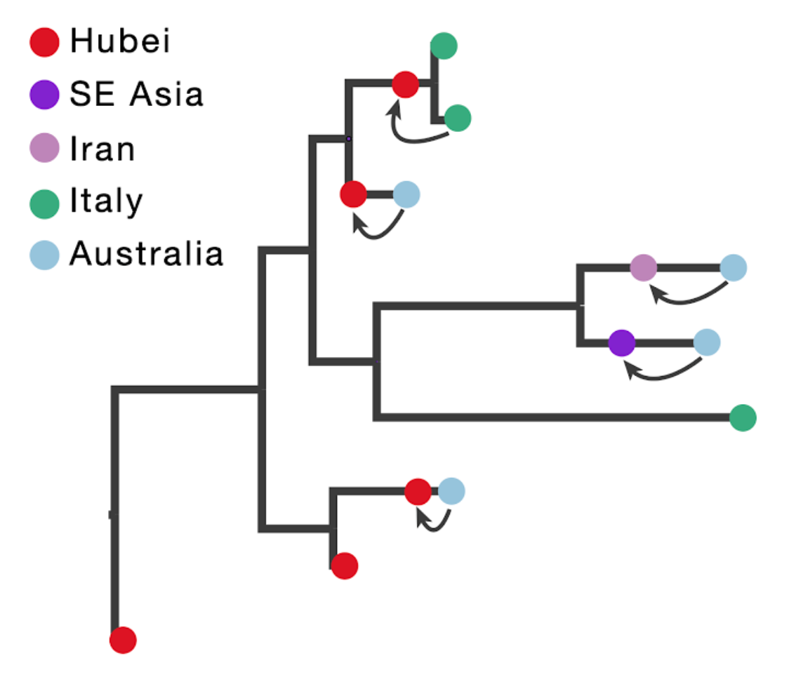
When a sampled traveller returned from location of origin to her/his destination, we take note of the time when the traveller started the return journey to her/his destination. At this time point in the ancestral path of the tip (indicated with arrows for the 5 relevant tips), we introduce an ancestral node and associate it with the location of origin in order to inform the reconstruction that at this point in time the lineage was in that location. The upper arrow in the figure above represents the information introduced for the traveller that returned from Hubei to Italy. The same procedure is applied to the four genomes from travellers returning to Australian from Hubei, Iran, Southeast Asia and Hubei again (from top to bottom in the figure above).
To specify this information in the XML, the standard <treeModel> is still defined and passed along to a new <ancestralTraitTreeModel>:
<!-- Travel history: defining ancestral trait tree model: in this case times are defined since the tip height (relativeToTipHeight="true") -->
    <ancestralTraitTreeModel id="ancestralTraitTreeModel">
        <treeModel idref="treeModel"/>
        <ancestor>
            <taxon idref="Australia/NSW11/2020|EPI_ISL_413597|2020-03-02_ancestor_taxon"/>
            <parameter id="pseudoBranchLength1" value="0.000" lower="0.0"/>
            <ancestralPath relativeToTipHeight="true">
                <taxon idref="Australia/NSW11/2020|EPI_ISL_413597|2020-03-02"/>
                <parameter id="time1" lower="0.0" value="0.02739726"/>
            </ancestralPath>
        </ancestor>
        <ancestor>
            <taxon idref="Australia/NSW09/2020|EPI_ISL_413595|2020-02-28_ancestor_taxon"/>
            <parameter id="pseudoBranchLength2" value="0.000" lower="0.0"/>
            <ancestralPath relativeToTipHeight="true">
                <taxon idref="Australia/NSW09/2020|EPI_ISL_413595|2020-02-28"/>
                <parameter id="time2" lower="0.0" value="0.02739726"/>
            </ancestralPath>
        </ancestor>
        <ancestor>
            <taxon idref="Australia/VIC01/2020|EPI_ISL_406844|2020-01-25_ancestor_taxon"/>
            <parameter id="pseudoBranchLength3" value="0.000" lower="0.0"/>
            <ancestralPath relativeToTipHeight="true">
                <taxon idref="Australia/VIC01/2020|EPI_ISL_406844|2020-01-25"/>
                <parameter id="time3" lower="0.0" value="0.016438356"/>
            </ancestralPath>
        </ancestor>
        <ancestor>
            <taxon idref="Australia/QLD02/2020|EPI_ISL_407896|2020-01-30_ancestor_taxon"/>
            <parameter id="pseudoBranchLength4" value="0.000" lower="0.0"/>
            <ancestralPath relativeToTipHeight="true">
                <taxon idref="Australia/QLD02/2020|EPI_ISL_407896|2020-01-30"/>
                <parameter id="time4" lower="0.0" value="0.008219178"/>
            </ancestralPath>
        </ancestor>
        <ancestor>
            <taxon idref="Italy/INMI1-cs/2020|EPI_ISL_410546|2020-01-31_ancestor_taxon"/>
            <parameter id="pseudoBranchLength5" value="0.000" lower="0.0"/>
            <ancestralPath relativeToTipHeight="true">
                <taxon idref="Italy/INMI1-cs/2020|EPI_ISL_410546|2020-01-31"/>
                <parameter id="time5" lower="0.0" value="0.016438356"/>
            </ancestralPath>
        </ancestor>
    </ancestralTraitTreeModel>
The code shows how incorporating the travel history for 5 individuals (which are referenced through their taxon ID) leads to 5 <ancestor> XML elements being created in the <ancestralTraitTreeModel> XML block.
The travel history for an individual is then specified using the <ancestralPath> XML element, with a node height reflecting the travel time relative to the sampling time for the inserted ancestral node.
Before we go into more detail, notice that instead of providing a reference to <treeModel> in <markovJumpsTreeLikelihood>...</markovJumpsTreeLikelihood>, we have to provide a reference to the constructed <ancestralTraitTreeModel>:
    <markovJumpsTreeLikelihood id="loc.treeLikelihood" stateTagName="loc.states" useUniformization="true" saveCompleteHistory="true" logCompleteHistory="true">
        <attributePatterns idref="loc.pattern"/>
        <!-- Travel history: referring ancestral trait tree model instead of standard treeModel-->
        <ancestralTraitTreeModel idref="ancestralTraitTreeModel"/>
        <siteModel idref="loc.siteModel"/>
        <generalSubstitutionModel idref="loc.model"/>
        <generalSubstitutionModel idref="loc.model"/>
        <strictClockBranchRates idref="loc.branchRates"/>
    </markovJumpsTreeLikelihood>
We also note that the travel time can be treated as a random variable in case the time of travelling to the sampling location is not known (with sufficient precision). We make use of this ability for the genomes associated with a travel location but without a clear travel time. In this particular example, we apply this approach to the first two Australian samples. The other 3 samples are provided with the actual travel times, expressed as the number of days before these samples were taken: 6 and 3 days for the other 2 Australian samples, and 6 days for the Italian sample.
We formalize this in our Bayesian inference framework by specifying normal prior distributions on the travel times, informed by an estimate of time of infection and truncated to be positive (back-in-time) relative to sampling date. Specifically, we use a mean of 10 days before sampling based on a mean incubation time of 5 days (Lauer et al., 2020) and a constant ascertainment period of 5 days between symptom onset and testing (Ferguson et al., 2020), and a standard deviation of 3 days to incorporate the uncertainty on the incubation time. We apply such a prior distribution to the travel times of the two first Australian samples as follows:
    <prior id="prior">
        ...
        <!-- Travel history: priors on two uncertain ancestral times; the mean corresponds to 10 days, the standard deviation to approximately 3 days -->
        <normalPrior mean="0.02739726" stdev="0.006989097">
            <parameter idref="time1"/>
        </normalPrior>
        <normalPrior mean="0.02739726" stdev="0.006989097">
            <parameter idref="time2"/>
        </normalPrior>
        ...
    </prior>
To complete the XML specification, we add in the transition kernels required to estimate the travel times for these two Australian samples:
    <operators id="operators" optimizationSchedule="log">
    ...
    <!-- Travel history: sampling two uncertain ancestral times -->
        <scaleOperator scaleFactor="0.75" weight="0.05">
            <parameter idref="time1"/>
        </scaleOperator>
        <scaleOperator scaleFactor="0.75" weight="0.05">
            <parameter idref="time2"/>
        </scaleOperator>
    ...
    </operators>
Finally, to obtain the full Markov jump history using this approach, we replace the <treeModel> references in <treeLog> with ancestralTreeLikelihood:
    <logTree logEvery="10000" nexusFormat="true" fileName="9seqs_travelHistory.loc.history.trees" sortTranslationTable="true">
        <!-- Travel history: referring ancestral trait tree model instead of standard treeMdodel -->
        <ancestralTraitTreeModel idref="ancestralTraitTreeModel"/>
        <trait name="loc.states" tag="loc">
            <ancestralTreeLikelihood idref="loc.treeLikelihood"/>
        </trait>
        <markovJumpsTreeLikelihood idref="loc.treeLikelihood"/>
    </logTree>
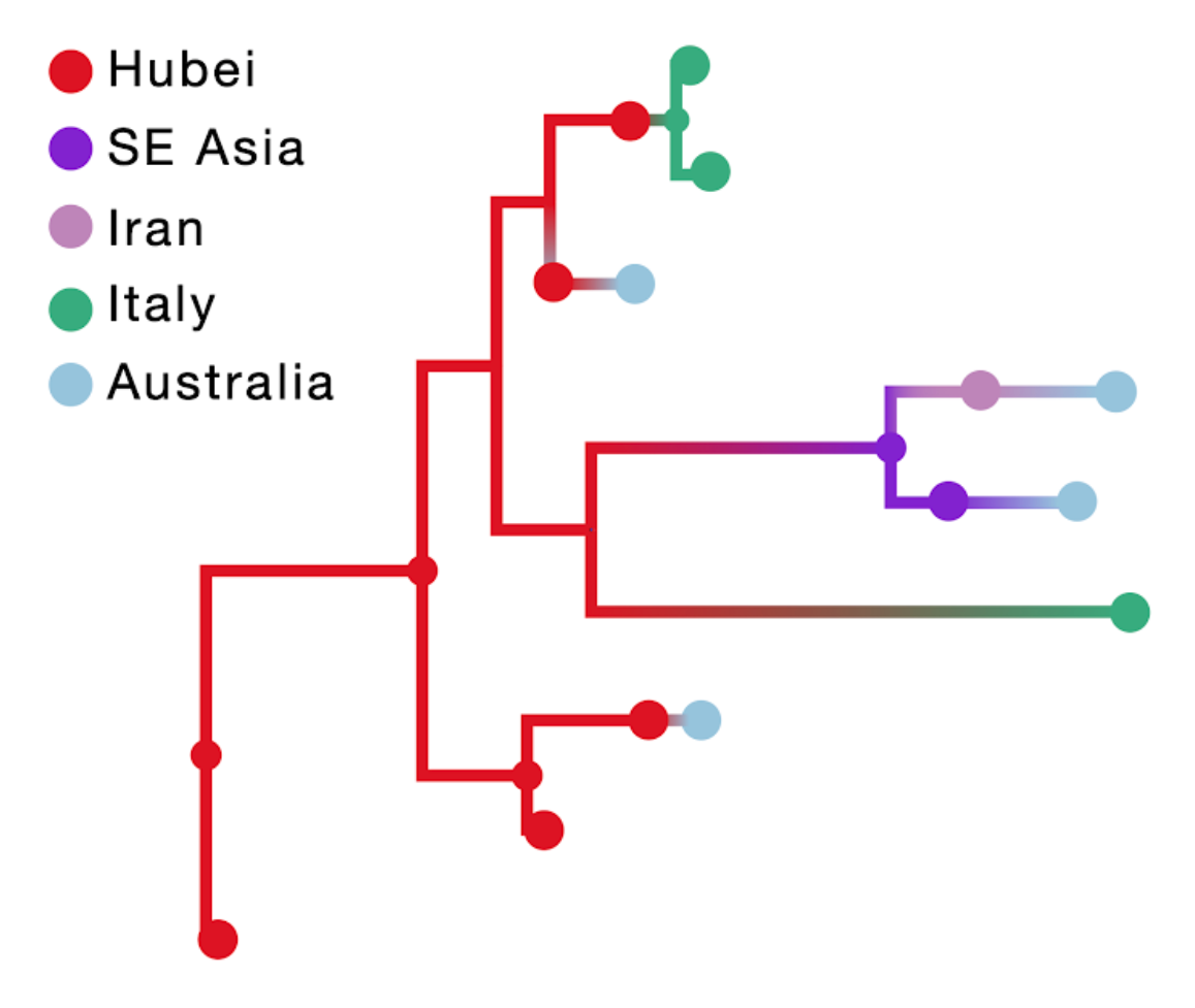
The result of this inference is shown in the figure below; the branch color reflects the modal state estimate at the child node. Incorporating travel history in discrete phylogeographic inference yields more realistic reconstructions of virus spread compared to currently available approaches.
Summarizing and visualizing phylogeographic estimates
In addition to the standard tools to summarize and visualize Bayesian phylogeographic estimates (e.g. TreeAnnotator, FigTree, spreaD3), we also make available a tool as part of BEAST to summarize the spatial trajectories in the ancestral history of specific taxa based on posterior tree distributions annotated with Markov jump histories.
As an example, we will look at the spatial trajectory of isolate EPI_ISL_413597 reconstructed under each phylogeographic model.
This is an isolate that was sampled in Australia, from a patient with a travel history to Iran.
We begin by extracting all Markov jump reconstructions for this taxon using the TaxaMarkovJumpHistoryAnalyzer tool, which is included in the latest BEAST jar file:
Usage: TaxonMarkovJumpHistory [-burnin <i>] [-taxaToProcess <list>] [-endState <end_state>] [-stateAnnotation <state_annotation_name>] [-mrsd <r>] [-help] <input-file-name> [<output-file-name>]
      -burnin the number of states to be considered as 'burn-in' [default = 0]
      -taxaToProcess a list of taxon names to process MJHs
      -endState a state at which the MJH processing stops
      -stateAnnotation The annotation name for the discrete state string
      -mrsd The most recent sampling time to convert heights to times [default=MAX_VALUE]
      -help option to print this message

  Example: taxonMarkovJumpHistory -taxaToProcess taxon1,taxon2 input.trees output.file
To extract all Markov jump histories for isolate EPI_ISL_413597 from the output of the travel history model, we type:
java -cp beast_travel_history.jar dr.app.tools.TaxaMarkovJumpHistoryAnalyzer -taxaToProcess 'Australia/NSW11/2020|EPI_ISL_413597|2020-03-02' -stateAnnotation loc -burnin 100 -mrsd 2020.1693989071039 9seqs_travelHistory.loc.history.trees EPI_ISL_413597.travelHistory.csv
We repeat the process with the trees obtained from the two remaining methods, to obtain a total of 3 CSV files containing the spatial histories reconstructed over each posterior tree distribution.
We can then use these files to visualize the spatial trajectories in the ancestral history of our taxon of interest by using a new R package we provide for this purpose (MarkovJumpR), available here.
This package can be installed in R via devtools::install_github("beast-dev/MarkovJumpR").
We can use the following R code to create a Markov jump trajectory plot for a given patient/sample/taxon:
library(MarkovJumpR)
library(lubridate)
# set up mapping of locations and colors
locations <- c("Wuhan","Italy","SEasia","Iran","Australia")
locationColors <-c("#E3272F","#31B186","#931ECF","#C695BD","#9DC7DD")
locationMap <- data.frame(
    location = locations,
    # ordering of countries in the plot
    position = c(1, 2, 3, 4, 5))

locationMap$color <- sapply(locationColors,as.character)

# load Markov jump history
travelHistPaths <- loadPaths(fileName = "EPI_ISL_413597.travel_hist.csv")
# set x-axis date labels
dateLabels <- c("01-Dec-19", "15-Dec-19", "01-Jan-20",
                "15-Jan-20", "01-Feb-20", "15-Feb-20", "01-Mar-20" )
# plot trajectories
plotPaths(travelHistPaths$paths, locationMap = locationMap,
          yJitterSd = 0.1, alpha = 0.1, minTime = 2019.9,
          addLocationLine = TRUE,
          xAt = decimal_date(dmy(dateLabels)),
          xLabels = dateLabels,
          mustDisplayAllLocations = TRUE)
Such a Markov jump trajectory plot depicts the posterior spatiotemporal ancestral transition history between locations from the sampling location of a specific taxon/sample (top of the plot) to the location of origin as inferred from the data set (bottom of the plot). Each trajectory plot summarizes across the posterior distribution (with Markov jump history annotation) the time intervals in the phylogenetic ancestry during which the virus remains in the same location (horizontal lines) and the transitions between two locations (vertical lines). The relative density of lines reflects the posterior uncertainty in location state and transition time between states.
We can compare these different Markov jump trajectory plots to assess the ancestral state reconstructions under each model:
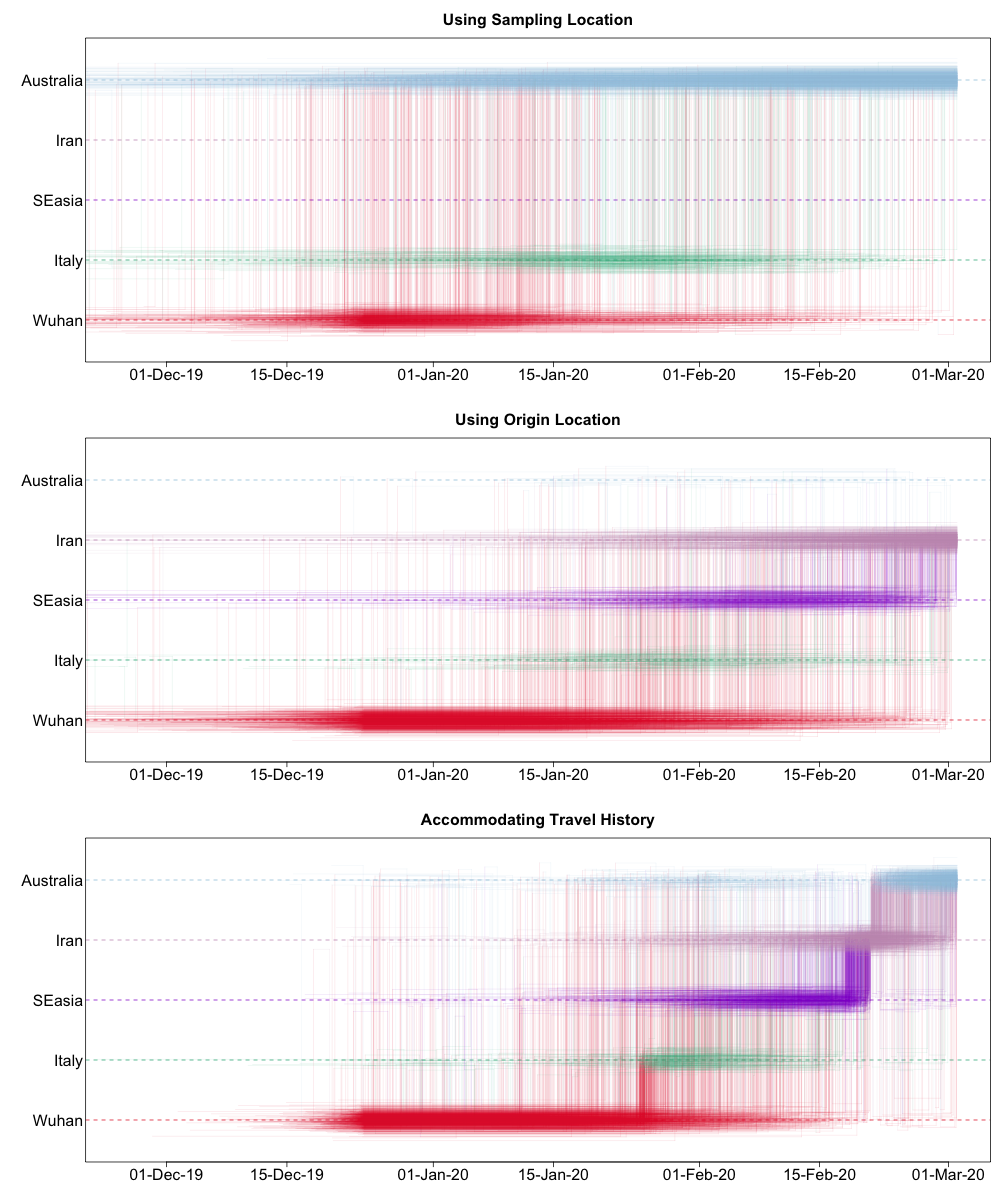
We can see from this plot that sampling location alone does not provide any support for Iranian ancestry, since the dataset does not include any genomes directly sampled from Iran. On the other hand, when using the locations of origin as tip locations, we see support for Iranian ancestry, but with considerable ambiguity. However, when we accommodate known travel history directly into the phylogeographic model, we not only see clear support for an ancestry that includes Iran, but also less variation in the spatial trajectories reconstructed.
References
- P. Lemey, A. Rambaut, A. J. Drummond, and M. A. Suchard. 2009. Bayesian phylogeography finds its roots. PLoS Computational Biology 5:e1000520.
- P. Lemey, S. Hong, V. Hill, G. Baele, C. Poletto, V. Colizza, A. O’Toole, J. T. McCrone, K. G. Andersen, M. Worobey, M. I. Nelson, A. Rambaut, and M. A. Suchard. 2020. Accommodating individual travel history, global mobility, and unsampled diversity in phylogeography: a SARS-CoV-2 case study. Submitted.
- M. A. Suchard, P. Lemey, G. Baele, D. L. Ayres, A. J. Drummond, and A. Rambaut. 2018. Bayesian phylogenetic and phylodynamic data integration using BEAST 1.10. Virus Evolution 4(1):vey016.
- S. A. Lauer, K. H. Grantz, Q. Bi, F. K. Jones, Q. Zheng, H. R. Meredith, A. S. Azman, N. G. Reich, and J. Lessler. 2020. The incubation period of coronavirus disease 2019 (COVID-19) from publicly reported confirmed cases: estimation and application. Annals of Internal Medicine 172:577-582.
- N. M. Ferguson, D. Laydon, G. Nedjati-Gilani, N. Imai, K. Ainslie, M. Baguelin, S. Bhatia, A. Boonyasiri, Z. Cucunubá, G. Cuomo-Dannenburg, A. Dighe, I. Dorigatti, H. Fu, K. Gaythorpe, W. Green, A. Hamlet, W. Hinsley, L. C. Okell, S. van Elsland, H. Thompson, R. Verity, E. Volz, H. Wang, Y. Wang, P. G. T. Walker, C. Walters, P. Winskill, C. Whittaker, C. A. Donnelly, Steven Riley, A. C. Ghani. 2020. Report 9: Impact of non-pharmaceutical interventions (NPIs) to reduce COVID-19 mortality and healthcare demand.
Help and documentation
The BEAST website: http://beast.community
Tutorials: http://beast.community/tutorials
Frequently asked questions: http://beast.community/faq