Model Selection Tutorial | BEAST Documentation

Model selection using path sampling / stepping-stone sampling in BEAST.

Marginal likelihood estimation using path sampling and stepping-stone sampling

Recent years have seen the development of several new approaches to perform model selection in the field of phylogenetics, such as path sampling (under the term ‘thermodynamic integration’; Lartillot and Philippe, 2006), stepping-stone sampling (Xie et al., 2011) and generalized stepping-stone sampling (Fan et al., 2011), with the latter approach currently only applicable on a fixed underlying topology. In a recently published paper in Molecular Biology and Evolution (Baele et al., 2012), the performance of 4 model selection approaches for demographic and molecular clock model comparison is investigated: the harmonic mean estimator (HME; Newton and Raftery, 1994), a posterior simulation-based analogue of Akaike’s information criteration (AICM; Raftery et al., 2007), path sampling (PS) and stepping-stone sampling. Baele et al. (2012) ‘confirm that the HME systematically overestimates the marginal likelihood and fails to yield reliable model classification and show that the AICM performs better and may be a useful initial evaluation of model choice but that it is also, to a lesser degree, unreliable’. The authors show ‘that path sampling and stepping-stone sampling substantially outperform these estimators’.

The publication is accompanied by 2 example BEAST XML files to indicate how to use the different estimators in BEAST, which is also what this tutorial focuses on. Below the mcmc block is provided of the BEAST XML example for a Bayesian skyline plot model (BSP) and an uncorrelated relaxed clock model with an underlying lognormal distribution (UCLD). This code runs an MCMC chain for 100 million iterations and stores samples from this chain in an output file. Besides collecting these samples, the definitions of prior and posterior in the code below are used when calculating the marginal likelihood using path sampling and stepping-stone sampling. As shown in Baele et al. (2013), it is important to specify proper priors for all the parameters being estimated in the analyses, especially to avoid convergence issues and numerical problems when performing path sampling (PS) and stepping-stone sampling (SS), although it is generally considered to be good practice in any case:

Note: As of BEAST v1.10, the <posterior id="posterior"> XML element has been renamed to a <joint id="joint"> XML element. Both will however remain valid but cannot be used interchangeably, i.e. we suggest you pick one of the two and stick with your choice throughout the entire XML.

<beast>
    <mcmc id="mcmc" chainLength="100000000" autoOptimize="true">
        <posterior id="posterior">
            <prior id="prior">
                <logNormalPrior mean="1.0" stdev="1.25" offset="0.0" meanInRealSpace="false">
                    <parameter idref="kappa"/>
                </logNormalPrior>
                <exponentialPrior mean="0.3333333333333333" offset="0.0">
                    <parameter idref="ucld.stdev"/>
                </exponentialPrior>
                <ctmcScalePrior>
                    <ctmcScale>
                        <parameter idref="ucld.mean"/>
                    </ctmcScale>
                    <treeModel idref="treeModel"/>
                </ctmcScalePrior>
                <logNormalPrior mean="1.0" stdev="1.5" offset="0.0" meanInRealSpace="false">
                    <parameter idref="constant.popSize"/>
                </logNormalPrior>
                <coalescentLikelihood idref="coalescent"/>
            </prior>
            <likelihood id="likelihood">
                <treeLikelihood idref="treeLikelihood"/>
            </likelihood>
        </posterior>
        ...
         <!-- write log to file -->
        <log id="fileLog" logEvery="1000" fileName="intergenic_UCLD_con.log">
            <posterior idref="posterior"/>
            <prior idref="prior"/>
            <likelihood idref="likelihood"/>
            <parameter idref="treeModel.rootHeight"/>
            <parameter idref="constant.popSize"/>
            <parameter idref="kappa"/>
            <parameter idref="ucld.mean"/>
            <parameter idref="ucld.stdev"/>
            <rateStatistic idref="meanRate"/>
            <rateStatistic idref="coefficientOfVariation"/>
            <rateCovarianceStatistic idref="covariance"/>
            <treeLikelihood idref="treeLikelihood"/>
            <coalescentLikelihood idref="coalescent"/>
        </log>
        ...
    </mcmc>
</beast>

Path sampling and stepping-stone sampling

Path sampling and stepping-stone sampling require additional calculations to perform model selection. Both approaches use the same collection of samples to estimate the marginal likelihood but do so in a different way. They both construct a path between prior and posterior (both defined in the mcmc block above) but, since path sampling uses Simpson’s triangulation formula, it converges less quickly to the true value than does stepping-stone sampling. However, when a lot of samples along this path are collected, this difference becomes negligible.

Note: while the HME and AICM are available in Tracer, path sampling and stepping-stone sampling are not, as they require additional calculations.

BEAUti

Path sampling and stepping-stone sampling can be set up in BEAUti, resulting in a set of power posteriors to be explored and sampled by BEAST. The collected samples will be used to construct both the path sampling and the stepping-stone sampling estimator for the log marginal likelihood. In other words, one set of additional calculations will result in two log marginal likelihood estimates and both will be printed to screen.

There is also a tutorial available on how to set up log marginal likelihood estimation using generalized stepping-stone sampling.

In BEAUti, and after loading a data set, go to the ‘MCMC’ panel. At the bottom, you can select your method of choice to estimate the log marginal likelihood for your selection of models on this data set. By default, no (log) marginal likelihood estimation will be performed and the option ‘None’ will be selected.

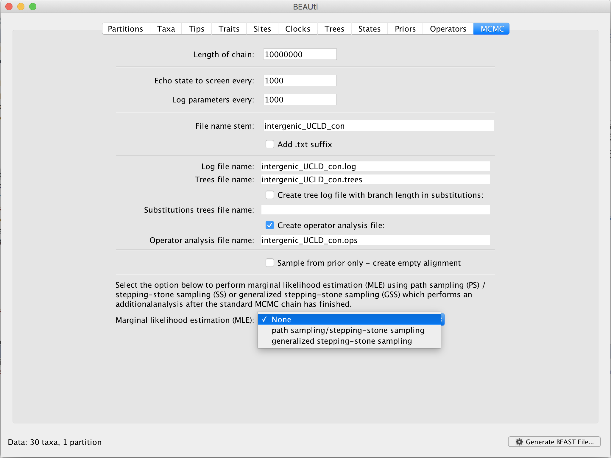
Upon selecting ‘path sampling/stepping-stone sampling’, clicking the ‘Settings’ button will open a new window where the settings for the log marginal likelihood estimation can be entered.

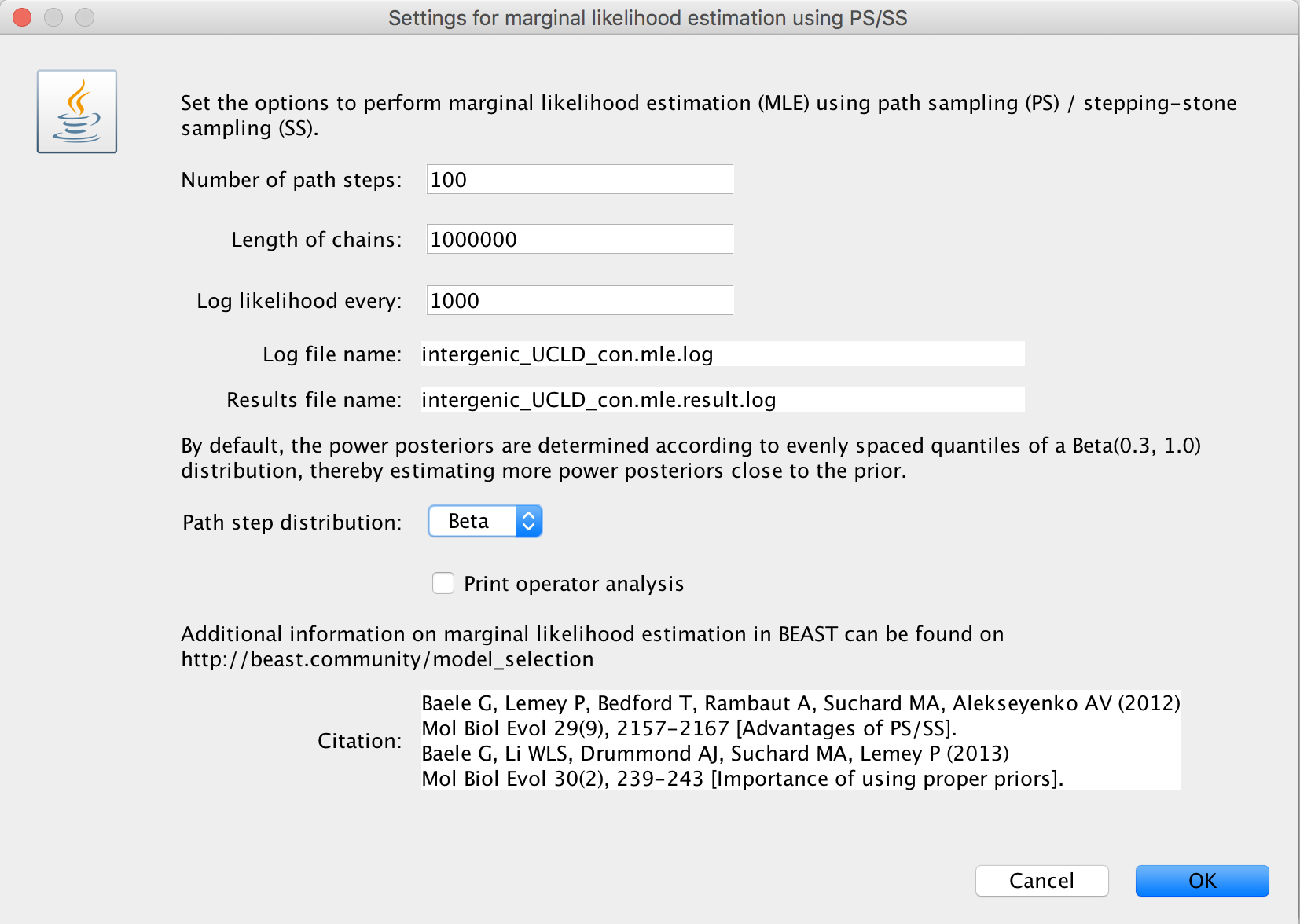
We suggest to specify a number of path steps of either 50 or 100, with the lenght of each chain being at least 250.000 iterations. In general, it’s probably a good idea to run a total amount of iterations (i.e. number of path steps times chain length) equal to the length of the standard BEAST analysis performed to estimate the various parameters. Given that the Beta(0.3; 1.0) distribution to determine the power posteriors has been shown to deliver adequate performance (Xie et al., 2011), we currently only allow this distribution to be used. Through XML specification (see below), other options for this distribution can be specified.

XML Specification

The XML code below, to be entered after the <mcmc> block (but still within the <beast> tags), runs a series of 100 power posteriors along the path between prior en posterior, with the powers being determined according to evenly spaced quantiles of a Beta(0.3,1.0) distribution:

<beast>
    <marginalLikelihoodEstimator chainLength="1000000" pathSteps="100" pathScheme="betaquantile" 
            alpha="0.30">
        <samplers>
            <mcmc idref="mcmc"/>
        </samplers>
        <pathLikelihood id="pathLikelihood">
            <source>
                <posterior idref="posterior"/>
            </source>
            <destination>
                <prior idref="prior"/>
            </destination>
        </pathLikelihood>
        <log id="MLE.con" logEvery="1000" fileName="MLE.con.log">
            <pathLikelihood idref="pathLikelihood"/>
        </log>
    </marginalLikelihoodEstimator>
</beast>

The samples collected from the power posteriors are stored in the MLE.bsp.log file, which is subsequently used as input for calculating the marginal likelihood using path sampling and stepping-stone sampling. The following code runs the path sampling calculation on the samples collected in the marginalLikelihoodEstimator element:

<beast>
    <pathSamplingAnalysis fileName="MLE.con.log">
        <likelihoodColumn name="pathLikelihood.delta"/>
        <thetaColumn name="pathLikelihood.theta"/>      
    </pathSamplingAnalysis>
</beast>

The code below then runs the stepping-stone sampling calculation on the same collection of samples gathered in the marginalLikelihoodEstimator element:

<beast>
    <steppingStoneSamplingAnalysis fileName="MLE.con.log">
        <likelihoodColumn name="pathLikelihood.delta"/>
        <thetaColumn name="pathLikelihood.theta"/>      
    </steppingStoneSamplingAnalysis>
</beast>

It is also possible to run several independent marginal likelihood calculations to obtain a larger number of samples to increase the accuracy of path sampling and stepping-stone sampling. For example, running the code above twice would result in two output files (e.g. MLE-1.bsp.log and MLE-2.bsp.log) containing different samples from a series of power posteriors. One can then combine these two output files (and hence the samples they contain) to estimate the marginal likelihood using path sampling and stepping-stone sampling by providing a list of the output files to the pathSamplingAnalysis and steppingStoneSamplingAnalysis XML elements. The following code runs the path sampling calculation on the two output files:

<beast>
    <pathSamplingAnalysis fileName="MLE-1.con.log MLE-2.con.log">
        <likelihoodColumn name="pathLikelihood.delta"/>
        <thetaColumn name="pathLikelihood.theta"/>      
    </pathSamplingAnalysis>
</beast>

The code below then runs the stepping-stone sampling calculation on these two output files:

<beast>
    <steppingStoneSamplingAnalysis fileName="MLE-1.con.log MLE-2.con.log">
        <likelihoodColumn name="pathLikelihood.delta"/>
        <thetaColumn name="pathLikelihood.theta"/>      
    </steppingStoneSamplingAnalysis>
</beast>

Note that if the two output files were obtained using independent runs, a separate BEAST XML file to combine these samples can easily be created. This XML file has no need for an mcmc or marginalLikelihoodEstimator block, since all the samples have already been collected and hence, no additional calculations are required.

HME, sHME and AICM (not recommended)

Warning: Given the poor performance and reliability of the HME and AICM, these estimators have been deprecated in the Tracer code base and will hence no longer be available in future versions of Tracer. For reliable and accurate marginal likelihood estimation, use path sampling and stepping-stone sampling or generalized stepping-stone sampling.

Note: marginal likelihood estimation using path sampling, stepping-stone sampling or generalized stepping-stone sampling cannot be performed in Tracer. Additional calculations are necessary to perform accurate model selection, and will be performed by BEAST.

XML Specification

Through XML specification, the estimation of the HME, sHME and AICM will still be supported in future versions of BEAST.

The following code runs the harmonic mean estimation on the samples collected in the mcmc and hence does not require additional calculations to be performed in order to estimate the marginal likelihood, which is considered a major advantage of this approach.

Note: given that additional model selection approaches are available as of BEAST v1.7.0, the mcmc element for the harmonic mean estimator is now assumed to be the following for clarity purposes (although the previous XML-element is still supported):

<beast>
    <harmonicMeanAnalysis fileName="intergenic_UCLD_con.log" bootstrapLength="0" burnIn="10000000">
        <likelihoodColumn name="likelihood" />
    </harmonicMeanAnalysis>
</beast>

The smoothed harmonic mean estimation (sHME) on the samples collected in the mcmc is run as follows:

<beast>
    <harmonicMeanAnalysis fileName="intergenic_UCLD_con.log" bootstrapLength="0" burnIn="10000000" 
            smoothedEstimate="true">
        <likelihoodColumn name="likelihood" />
    </harmonicMeanAnalysis>
</beast>

Another approach that is able to perform model selection using the samples collected during the MCMC run is the AICM.

Note: the AICM is NOT a marginal likelihood estimator. The AICM estimation on the samples collected in the mcmc is run using the following code:

<beast>
    <aicmAnalysis fileName="intergenic_UCLD_con.log" bootstrapLength="0" burnIn="10000000">
        <likelihoodColumn name="likelihood" />
    </aicmAnalysis>
</beast>

Citations

If you use this code we would encourage you to cite the following papers:

G. Baele, P. Lemey, T. Bedford, A. Rambaut, M. A. Suchard, M. A. and A. V. Alekseyenko (2012) Improving the accuracy of demographic and molecular clock model comparison while accommodating phylogenetic uncertainty. Mol. Biol. Evol. 29(9), 2157-2167.

G. Baele, W. L. S. Li, A. J. Drummond, M. A. Suchard, and P. Lemey (2013) Accurate model selection of relaxed molecular clocks in Bayesian phylogenetics. Mol. Biol. Evol. 30(2):239-243.

If you’d like to know more about the use of path sampling (PS) and stepping-stone sampling (SS) on whole genome data sets (i.e. involving a lot of parameters across different genes) and/or using multi-core hardware in BEAST/BEAGLE, we’d like to refer you to the following paper:

G. Baele and P. Lemey (2013) Bayesian evolutionary model testing in the phylogenomics era: matching model complexity with computational efficiency. Bioinformatics 29(16):1970-1979.

The following paper is a more technical paper on performing direct (log) Bayes factor estimation between two models using path sampling (PS) and stepping-stone sampling (SS), with an emphasis on the derivation of the statistical properties of the latter. This paper focuses on comparing high-dimensional substitution models, but currently does not offer a BEAST implementation:

G. Baele, P. Lemey and S. Vansteelandt (2013) Make the most of your samples: Bayes factor estimators for high-dimensional models of sequence evolution. BMC Bioinformatics 14:85.

References

N. Lartillot and H. Philippe (2006) Computing Bayes factors using thermodynamic integration. Syst. Biol. 55:195–207.

W. Xie, P. O. Lewis, Y. Fan, L. Kuo and M. H. Chen (2011). Improving marginal likelihood estimation for Bayesian phylogenetic model selection. Syst. Biol. 60:150–160.

Y. Fan, R. Wu, M. H. Chen, L. Kuo and P. O. Lewis (2011) Choosing among partition models in Bayesian phylogenetics. Mol. Biol. Evol. 28:523–532.

M. A. Newton and A. E. Raftery (1994) Approximating Bayesian inference with the weighted likelihood bootstrap. J. R. Stat. Soc. B 56:3–48.

A. E. Raftery, M. A. Newton, J. Satagopan and P. Krivitsky (2007) Estimating the integrated likelihood via posterior simulation using the harmonic mean identity. In: Bernardo JM, Bayarri MJ, Berger JO, editors. Bayesian Statistics. Oxford: Oxford University Press. p. 1–45.

Tags: