Ebola Virus Local Clock Analysis
In 2014 there was an outbreak of Ebola virus disease in the Democratic Republic of Congo. When the first genome sequences were published (Maganga et al. 2014) it was noticed that the amount of divergence from the earliest EBOV genomes from the 1970s was considerably less than for the West African epidemic genomes which were from the same year. This suggested that the DRC lineage had exhibited a substantially lower rate of evolution (Lam et al. 2015). Lam et al. speculated that this may be due to it being in a different host species with different evolutionary forces at work.
However, during the West African outbreak, a number of examples of long-term latency were observed where someone who had recovered from EVD months later transmitted the virus to another individual – usually a sexual partner (Blackley et al. 2016). In the most extreme example, there was a 15 month interval between the acute infection and the onward transmission (Diallo et al. 2016). It was noticed that these cases were often associated with a short branch length suggesting a reduced rate of evolution or a form of latency with reduced replication for much of the period. This suggests that a similar process could be at work for EBOV in the non-human animal hosts over longer timescales.
Sequences from the last 3 DRC outbreaks (in 2017, summer 2018 and the currently ongoing one in the North East of the country) also exhibit this apparently reduced branch length. See this post for a tree produced by the INRB and USAMRIID that shows this effect and also Mbala-Kingebeni et al. 2019b.
To explore EBOV rate varation in non-human hosts, we assembled a data set of genomes that spans the known history of the virus. Most EBOV genomes have been sampled from human cases so we have included one genome per outbreak, preferring those with precise dates of sampling. A list of sequences used is given in Table 1 along with their Genbank accession numbers and, where available, a reference to the published work describing them.
| accession | country | name | date | outbreak | reference |
|---|---|---|---|---|---|
| KR063671 | DRC | Yambuku-Mayinga | 1976-10-01 | Yambuku/1976 | |
| KC242791 | DRC | Bonduni | 1977-06 | Bonduni/1977 | Carroll et al. 2013 |
| KC242792 | GAB | Gabon | 1994-12-27 | Minkebe/1994 | Carroll et al. 2013 |
| KU182905 | DRC | Kikwit-9510621 | 1995-05-04 | Kikwit/1995 | |
| KC242793 | GAB | 1Eko | 1996-02 | Mayibout/1996 | Carroll et al. 2013 |
| KC242798 | GAB | 1Ikot | 1996-10-27 | Booue/1996 | Carroll et al. 2013 |
| KC242800 | GAB | Ilembe | 2002-02-23 | Mekambo/2001 | Carroll et al. 2013 |
| KF113529 | COG | Kelle_2 | 2003-10 | Mbomo/2003 | Chiu et al. 2013 |
| HQ613403 | DRC | M-M | 2007-08-31 | Luebo/2007 | Grard et al. 2011 |
| HQ613402 | DRC | 034-KS | 2008-12-31 | Luebo/2008 | Grard et al. 2011 |
| KJ660347 | GIN | Makona-Gueckedou-C07 | 2014-03-20 | West_Africa/2013 | Baize et al. 2014 |
| KP271018 | DRC | Lomela-Lokolia16 | 2014-08-20 | Boende-Lokolia/2014 | Naccache et al. 2014 |
| MH613311 | DRC | Muembe.1 | 2017-05-07 | Likati/2017 | Nsio et al. 2018 |
| MH733477 | DRC | Tumba-BIK009 | 2018-05-10 | Bikoro-Mbandaka/2018 | Mbala-Kingebeni et al. 2019a |
| MK007330 | DRC | Ituri-18FHV090 | 2018-07-28 | Kivu/2018 | Mbala-Kingebeni et al. 2019b |
Table 1 A list of the genomes used in this post and their references.
Building a maximum likelihood tree of these genomes shows the apparent slow down in the recent lineages (Figure 1; yellow dots). A root-to-tip regression (the line is fitted only to the green dots) shows how far below the expected line these are (this is similar to Figure 5 in Mbala-Kingebeni et al. 2019b).
Figure 1. A tree and root-to-tip plot for the 15 Ebola virus genomes in Table 1. This is an interactive figure: click the points to include/exclude them from the regression. The yellow tips are not included in the regression. Click on a branch of the tree to re-root the tree at that position. The source code for this figure is available here.
Methods
To characterise this effect, we have used relaxed-clock models in BEAST to allow different rates of evolution for different parts of the tree.
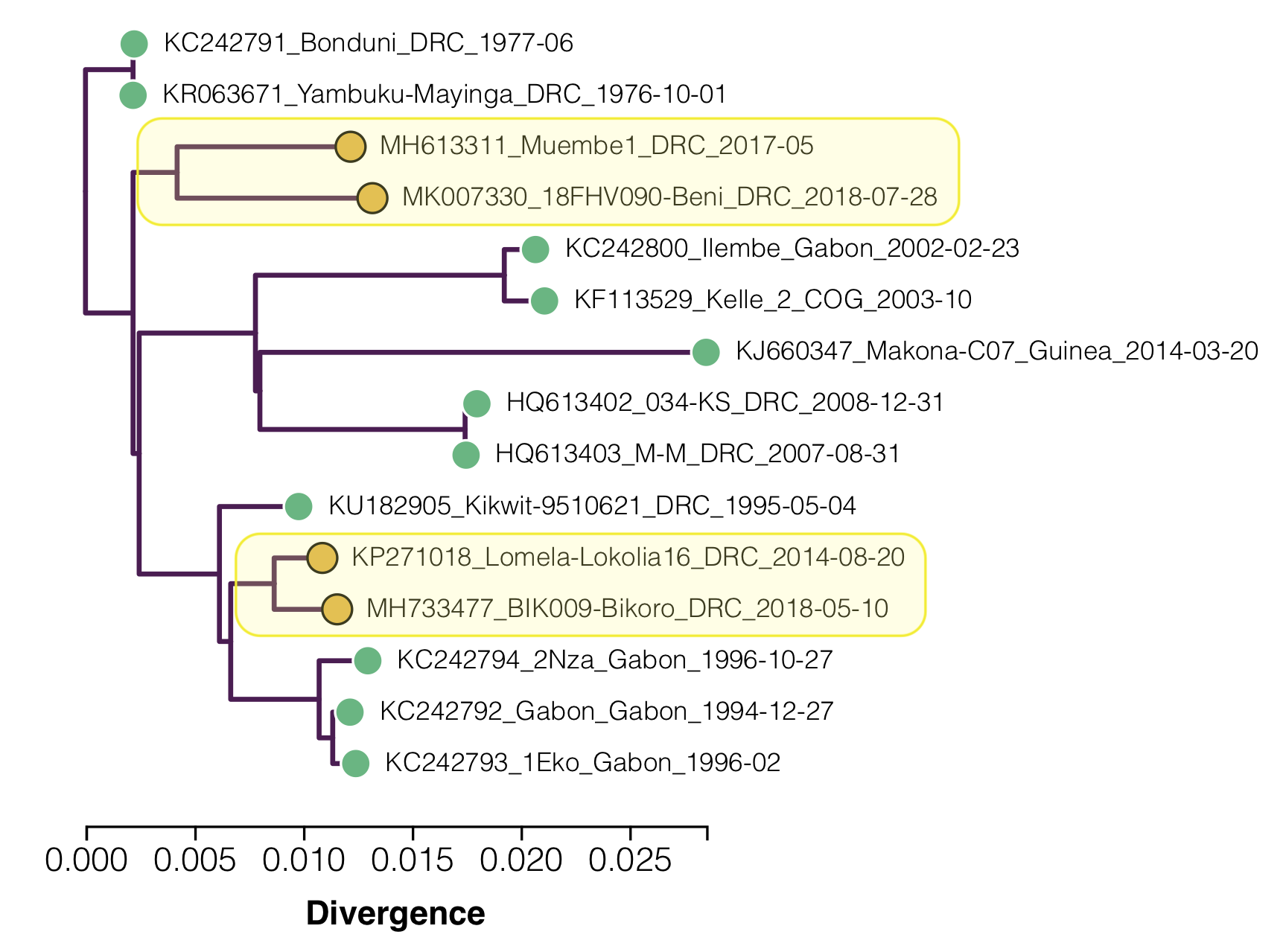
Figure 2. A maximum likelihood tree of the 15 EBOV genomes with the ‘slow’ clades highlighted.
Two lineages are identified as having lower than expected divergence by Mbala-Kingebeni et al. 2019b (see Figure 2):
- One comprising the outbreak in 2017 in Likati and the on-going 2018-2019 outbreak in North Kivu Province – represented by the genomes Muembe.1 and Ituri-18FHV090.
- The other comprising the outbreak in 2014 in Lokolia and the 2018 outbreak in Équateur Province – represented by the genomes Lomela-Lokolia16 and Tumba-BIK009.
Firstly we used the Local Clock model which allows us to specify which parts of the tree have different rates (although this doesn’t specify which bits are fast and which are slow). This allows us to assign a different rate of evolution to the two lineages described above (including the ‘stem’ branch leading to each clade).
This model was used in Mbala-Kingebeni et al. (2019b) where these two lineages are labelled clade a (“EBOV/Tum” & “EBOV/Lom”) and clade c (“EBOV/Muy” & “EBOV/Itu”), respectively (Figure S8 of the Supplementary information). This paper shows that both these clades have a lower rate of evolution over all (Figure S8B).
As a comparison we also ran the analysis with a strict molecular clock (which assumes a single rate over the whole tree) and a log-normal uncorrelated relaxed clock (which allows each branch to have a different rate, independently drawn from a log-normal distribution). We also ran a strict molecular clock but excluding the recent DRC outbreak genomes.
For all of these analyses we constrained the tree topology so all of the viruses after the 1970s were monophyletic to maintain a consistent rooting. This was the rooting suggested by a much earlier an analysis (Dudas and Rambaut 2014).
Analysis was done by partitioning the genomes into 1st, 2nd & 3rd codon positions for the concatenated protein coding regions and a 4th partition comprising the concatenated intergenic regions. Each partition was given an HKY model with gamma distributed site-specific rates and parameters for each were unlinked.
Results
For the local clock model (Figure 3), you can see the two lineages that have been allowed a different rate and both have a slower rate than the rest of the tree (i.e. the branches are coloured by rate with blue meaning lower than average). This and all the subsequent trees are drawn on the same timescale to allow a comparison of the depth of the trees.
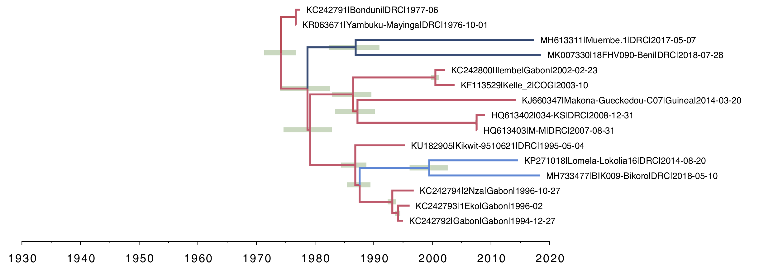
Figure 3. A local clock tree where two lineages, identified a priori, are allowed to evolve at a different rate. The branches are coloured by rate with blue meaning lower than average, red higher. Green bars represent 95% credible intervals for the date of the node.
Secondly, for the relaxed clock tree (Figure 4), you can see that there is variation in rate across the tree (the clades of interest do, however, have the slowest rates). Note however that the age of the root of the tree is further back in time and the HPD bar spans nearly 4 decades. Essentially the lognormal distribution is struggling to adequately describe the variation in rates given the extreme outliers seen in Figure 3.
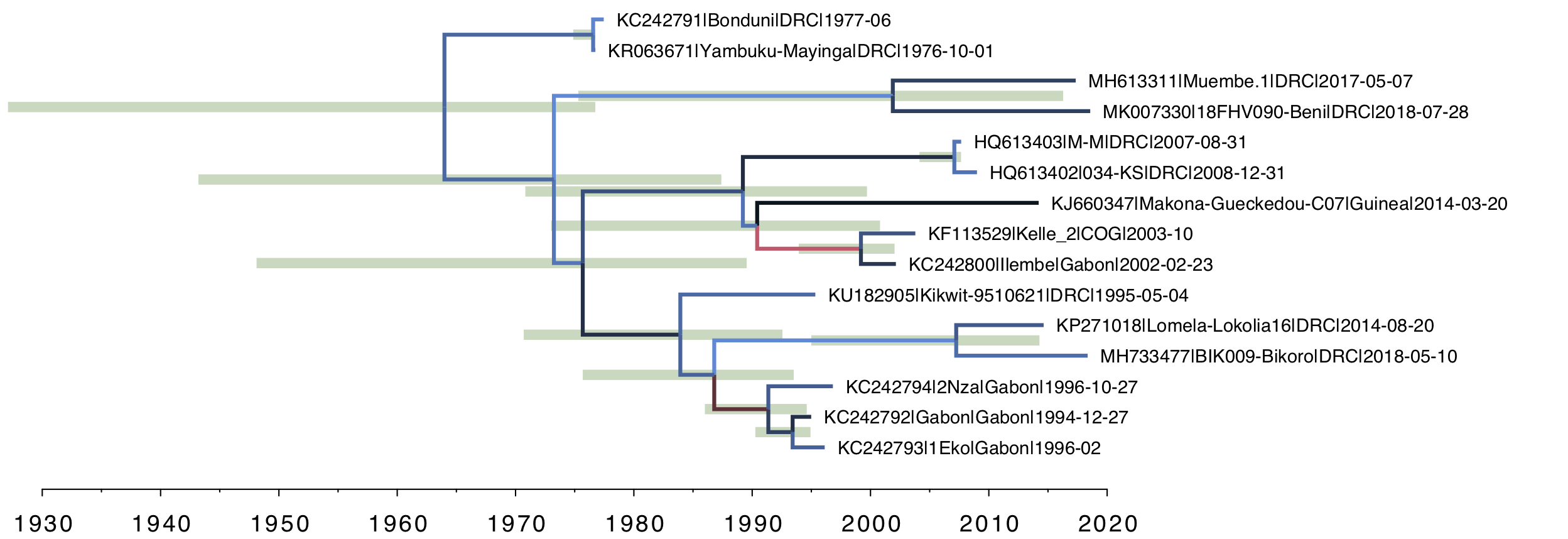
Figure 4. The uncorrelated lognormal (UCLN) relaxed clock model. The rate for each branch is inferred independently with no a priori structure imposed.
Finally, as a comparison, here is the strict molecular clock tree with the same rate over the whole tree (Figure 5). Once again, the root of the tree is much older than the local clock model and the relative branch lengths are very different.
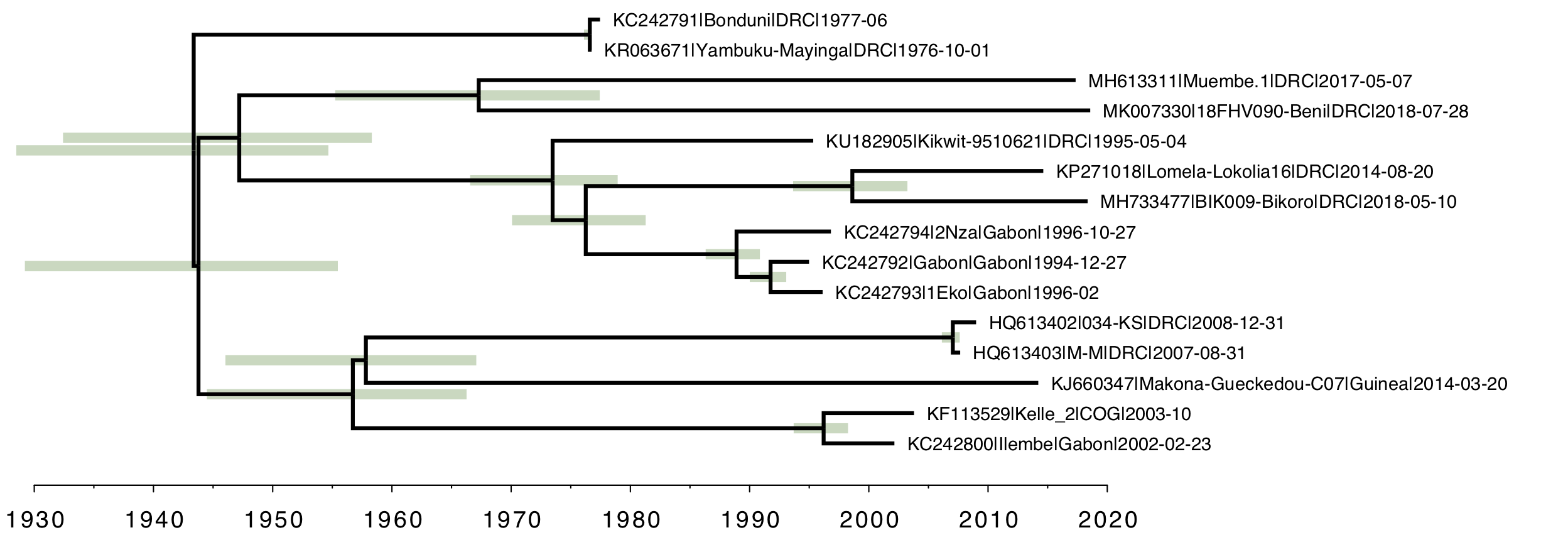
Figure 5. The strict molecular clock model with a single rate describing the whole tree.
Refining the model
Looking at the relaxed clock tree in Figure 4, we notice that for the two clades of interest, the tip branches seem to have a higher rate than the stem branches (they are less blue and they are shorter than in the local clock model). This suggests another possibility — that it is not the whole clade that has a lower rate of evolution but just the branch leading to the common ancestor of the pair. This makes more sense if this is being produced by a process of latency (i.e., a switch between active replication and no replication). This would mean that, parsimoniously, there were just these two branches where the virus was latent for some period of time. We would assume that an internal node in the tree represents active replication and epidemiological spread and thus the virus being in the non-latent state. Thus it is unlikely that a whole clade and stem exhibits latency (unless the propensity to latency increased on the stem lineage).
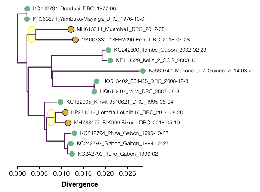
Figure 6. The two stem branches given a different rate of evolution in the refined local clock model (the rest of the tree is assumed to have the same rate including the tip branches of the two clades identified in Figure 2.
To examine this we can set up a new local clock model which just has the internal stem branch given the different rate of evolution with the tip branches in this clade having the same rate as the rest of the tree (Figure 6).
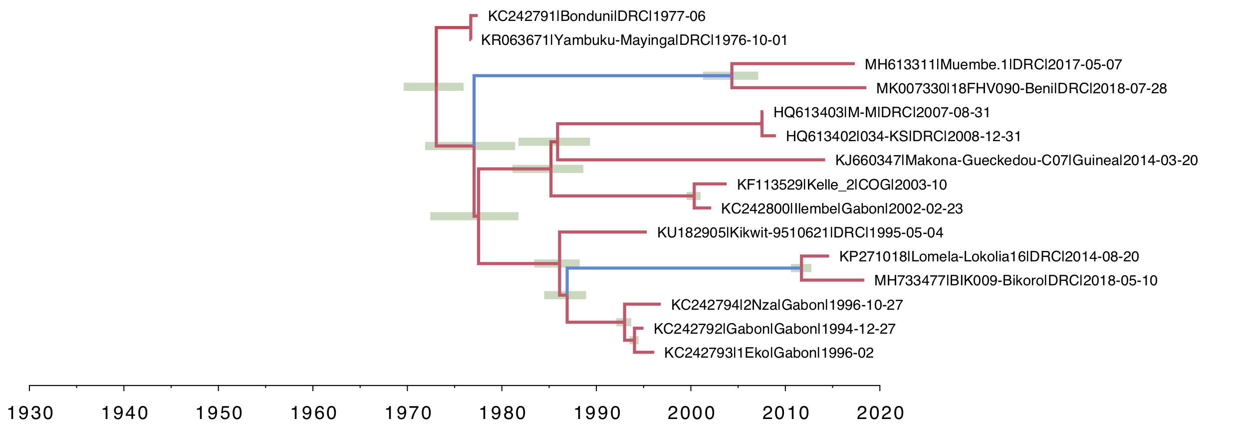
Figure 7. Stem branch only local clock model. Only the stem branches above the two clades of interest are allowed different rates of evolution.
In comparison with the clade-specific local clock (Figure 3), the most recent common ancestors of the Muembe.1/18FHV090 pair and Lokolia/Bikoro pair are much more recent. Other than that, the trees are very similar. The rates of evolution on the two stem lineages are even slower (more blue). We compare the actual values of these rates in Figure 9.
Looking at the average rate of evolution over the whole tree (Figure 8) shows the slow-down in the in the two lineages affects the strict clock to a much greater degree than the relaxed clocks.
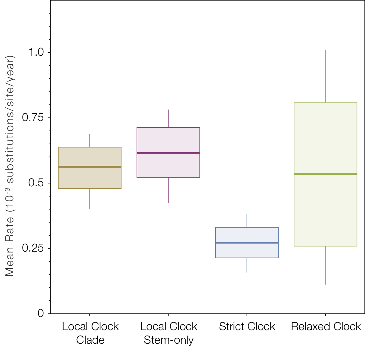
Figure 8. Box-and-whisker plot of the mean rates of evolution across all four models.
But if we look at the local clock models and compare the rates for the Likati/North Kivu and Lokolia/Équateur clades and the respective stem branches (Figure 9), we see the slow rates (the stem-only model gives an even slower rate for this one branch - supporting the idea that this is the branch that experienced some ‘latency’). Interestingly the rates for the two stem branches are even lower than the clades and very similar (whereas the rates for the clades are different because they include a mixture of fast and slow branches for different amounts of time).
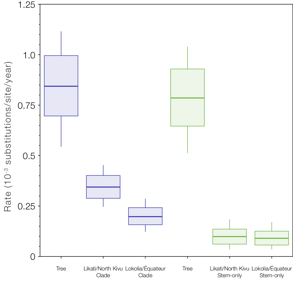
Figure 9. Box-and-whisker plot of the estimated rates for the two local clock model variants. The rate labelled ‘Tree’ is the rate for the rest of the tree (excluding the local clocks), then the rates for the Likati/North Kivu and Lokolia/Équateur lineages when the whole clade is included and then only the stem lineages.
Finally we ran the strict clock model on a data set where we omitted the four most recent DRC genomes that are involved in the apperent slow down in rates (the last 4 sequences in Table 1). We compared this rate with the two local clock models for the rate of evolution estimated for the parts of the tree that are not included in the local clocks (the red branches in Figures 3 and 7).
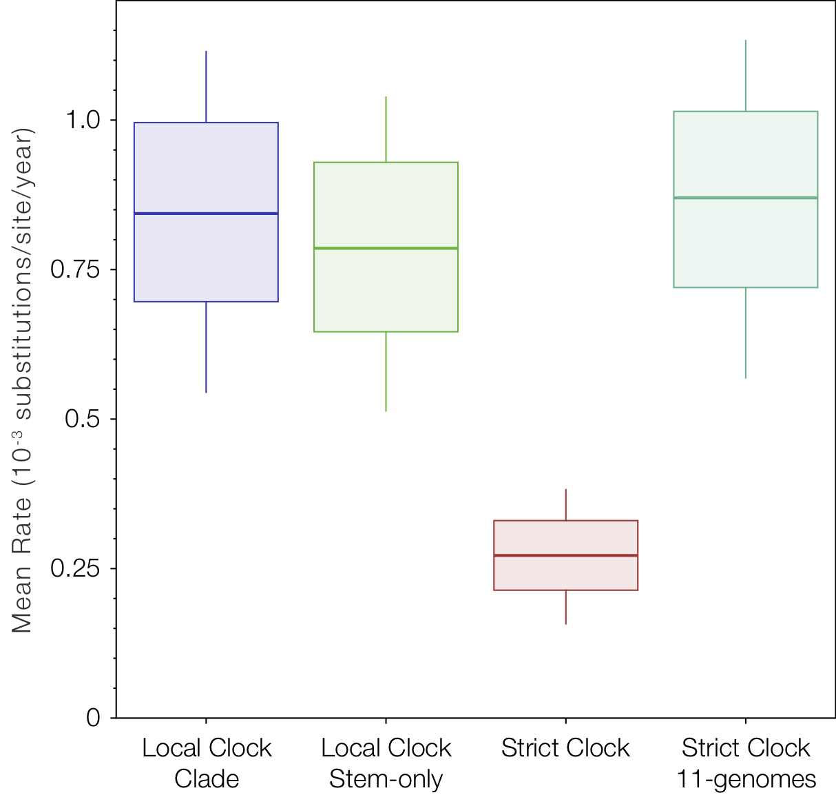
Figure 10. Box-and-whisker plot of the estimated rate for the tree (excluding the local clock rates for these models) in comparison to the strict clock rate and the rate for a strict clock on a data set that excludes the 4 recent DRC genomes (i.e., excluding the lineages that are exhibiting slow downs).
Model selection
BEAST implements a number of related approaches for comparing competing models (see here for some detailed instructions on applying these). These compute a marginal likelihood estimate - essentially a goodness-of-fit which takes into account the complexity of the models. The ratio of these provides a Bayes factor - a measure of the relative ‘plausibility’ of the models given the data.
| model | log MLE | log Bayes factor |
|---|---|---|
| strict clock | -33661.96 | — |
| clade local clock | -33566.74 | 95.22 (vs. strict clock) |
| stem local clock | -33563.86 | 2.88 (vs. clade local clock) |
| UCLN relaxed clock | -33539.62 | 24.24 (vs. stem local clock) |
Table 2 Marginal likelihood estimates (MLE) and Bayes factors for the models discussed here. The 3rd column gives the difference between the log MLE for the model and the model above which is the log Bayes factor for the two.
The uncorrelated lognormal relaxed clock (UCLN) is the best fitting model (by a good margin) as it clearly accommodates some of the ‘slow-down’ in the two stem branches but also other variation in rate across the tree (Figure 4). However, the time and rate estimates are very variable.
The good fit of the UCLN model suggests there is random variation in rate across the tree as well as the specific ‘latency’ slow downs. So we constructed a model that is a mix of the stem local clock and the UCLN — this essentially states that the two stem branches have their own rate and the rates for the rest of the tree are drawn from the lognormal relaxed clock (Figure 11).
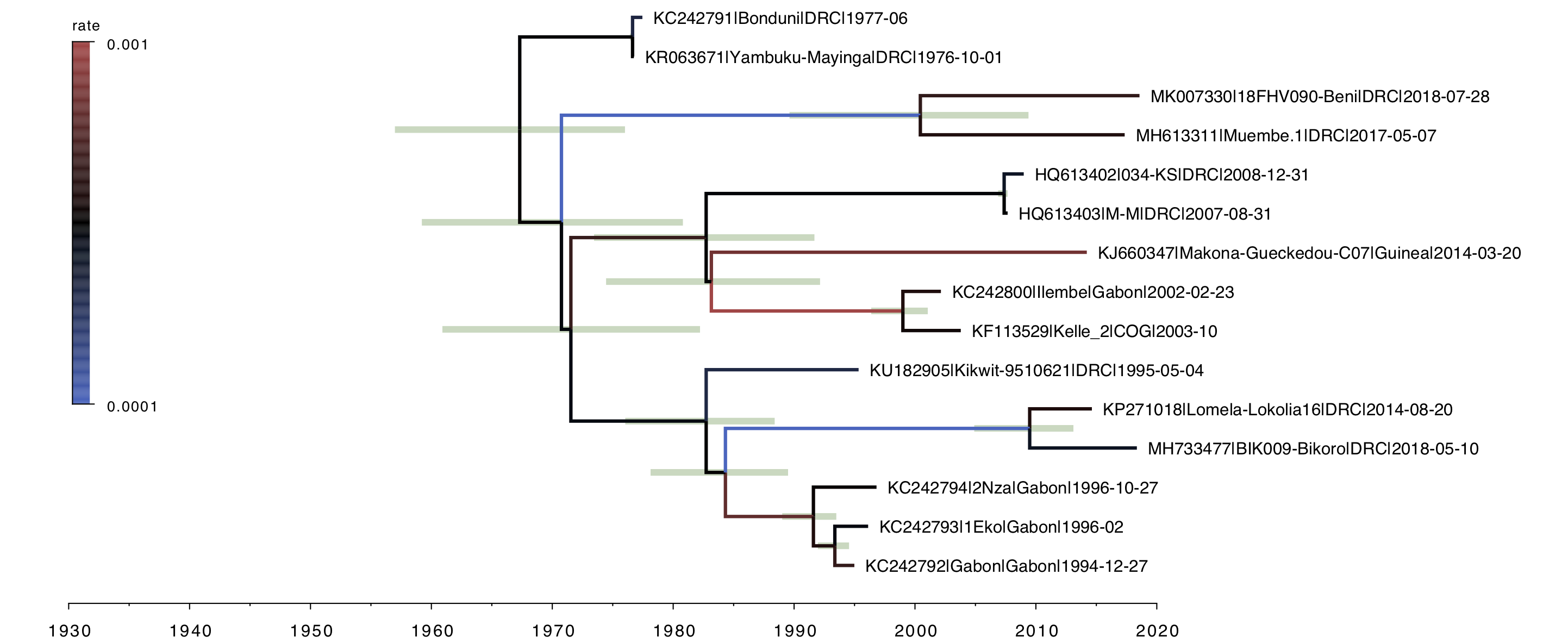
Figure 11. MCC tree constructed for the mix of the stem local clock model and the UCLN relaxed clock.
Over all this tree is quite similar to the straight UCLN one (Figure 4) but with much tighter credible (HPD) intervals on the node ages. This suggests overall better model fit (less of a struggle to fit competing patterns of rate variation). Indeed the MLE estimate for this model is -33536.59 giving a log Bayes factor of 3.03 (more than 20-fold) over the UCLN model. The rates are comparable (Figure 12) but as expected the addition of the relaxed clock gives more variation in these.
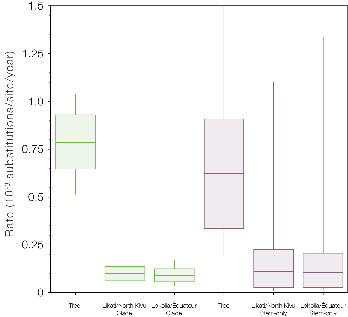
Figure 12. The rates for the tree and the two stem branches under the stem local clock model (left) and the stem local clock + relaxed clock model (right).
Final points
Although we forced the rooting of the tree to be the same for each model, it is likely that the strict clock model and the relaxed clock model would give a different rooting (and possibly rates) if the constraint was removed.
Finally, we are developing an explicit model of latency which will act as a molecular clock model, infer the branches that have evidence of latency and estimate parameters of the process. More on this soon.
References
Baize, S. et al., 2014. Emergence of Zaire Ebola Virus Disease in Guinea. The New England journal of medicine, 371(15), pp.1418–1425.
Carroll, S.A. et al., 2013. Molecular Evolution of Viruses of the Family Filoviridae Based on 97 Whole-Genome Sequences. Journal of virology, 87(5), pp.2608–2616.
Diallo, B. et al., 2016. Resurgence of Ebola Virus Disease in Guinea Linked to a Survivor With Virus Persistence in Seminal Fluid for More Than 500 Days. Clinical infectious diseases: an official publication of the Infectious Diseases Society of America, 63(10), pp.1353–1356. Grard, G. et al., 2011. Emergence of divergent Zaire ebola virus strains in Democratic Republic of the Congo in 2007 and 2008. The Journal of infectious diseases, 204 Suppl 3, pp.S776–84.
Lam, T.T.-Y. et al., 2015. Puzzling origins of the Ebola outbreak in the Democratic Republic of the Congo, 2014. Journal of virology, pp.JVI.01226–15. https://doi.org/10.1128/JVI.01226-15
Maganga, G.D. et al., 2014. Ebola Virus Disease in the Democratic Republic of Congo. The New England journal of medicine, 371(22), pp.2083–2091.
Mbala-Kingebeni, P., Pratt, C.B., et al., 2019. 2018 Ebola virus disease outbreak in Équateur Province, Democratic Republic of the Congo: a retrospective genomic characterisation. The Lancet infectious diseases. http://dx.doi.org/10.1016/S1473-3099(19)30124-0.
Mbala-Kingebeni, P., Aziza, A., et al., 2019. Medical countermeasures during the 2018 Ebola virus disease outbreak in the North Kivu and Ituri Provinces of the Democratic Republic of the Congo: a rapid genomic assessment. The Lancet infectious diseases. http://dx.doi.org/10.1016/S1473-3099(19)30118-5.
Nsio, J. et al., 2019. 2017 Outbreak of Ebola Virus Disease in Northern Democratic Republic of Congo. The Journal of infectious diseases. https://http://doi.org/10.1093/infdis/jiz107