Introduction
The first step will be to convert an alignment file in fasta format into a BEAST XML input file. This is done using the program BEAUti (this stands for Bayesian Evolutionary Analysis Utility). This is a user-friendly program for setting the evolutionary model and options for the MCMC analysis. The second step is to actually run BEAST using the input file that contains the data, model and settings. The final step is to explore the output of BEAST in order to diagnose problems and to summarize the results.
To undertake this tutorial, you will need to download three software packages in a format that is compatible with your computer system (all three are available for Mac OS X, Windows and Linux/UNIX operating systems):
EXERCISE 1: Host and location ancestral reconstruction
Running BEAUti
Loading the sequence data file
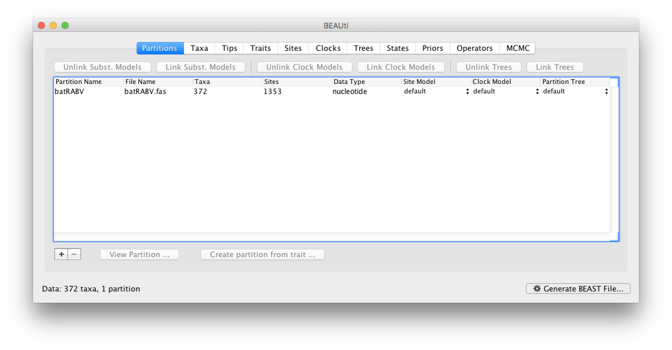
The input file for this tutorial, batRABV.fas, can be downloaded from here. This fasta formatted file contains an alignment of 372 nucleoprotein gene sequences of bat rabies viruses, 1353 nucleotides in length.
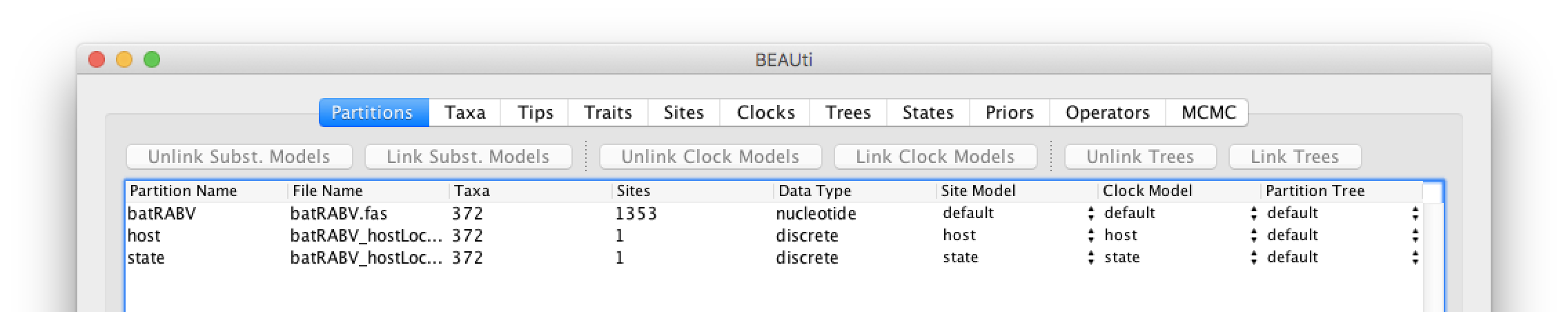
To load the alignment, simply select the Import Data... option from the File menu. Select the batRABV.fas file. Once loaded, the sequence data will be listed under Partitions as shown in the figure:
Specifying the sampling date information
By default all the taxa are assumed to have a date of zero (i.e. the sequences are assumed to be sampled at the same time). However, the RABV sequences have been sampled at various years going back to 1997. To set these dates switch to the Tips panel using the tabs at the top of the window.
Select the box labelled Use tip dates. The RABV sequences have their date of sampling encoded in their labels so use the Parse Dates button at the top of the Tips panel. Clicking this will make a dialog box appear:
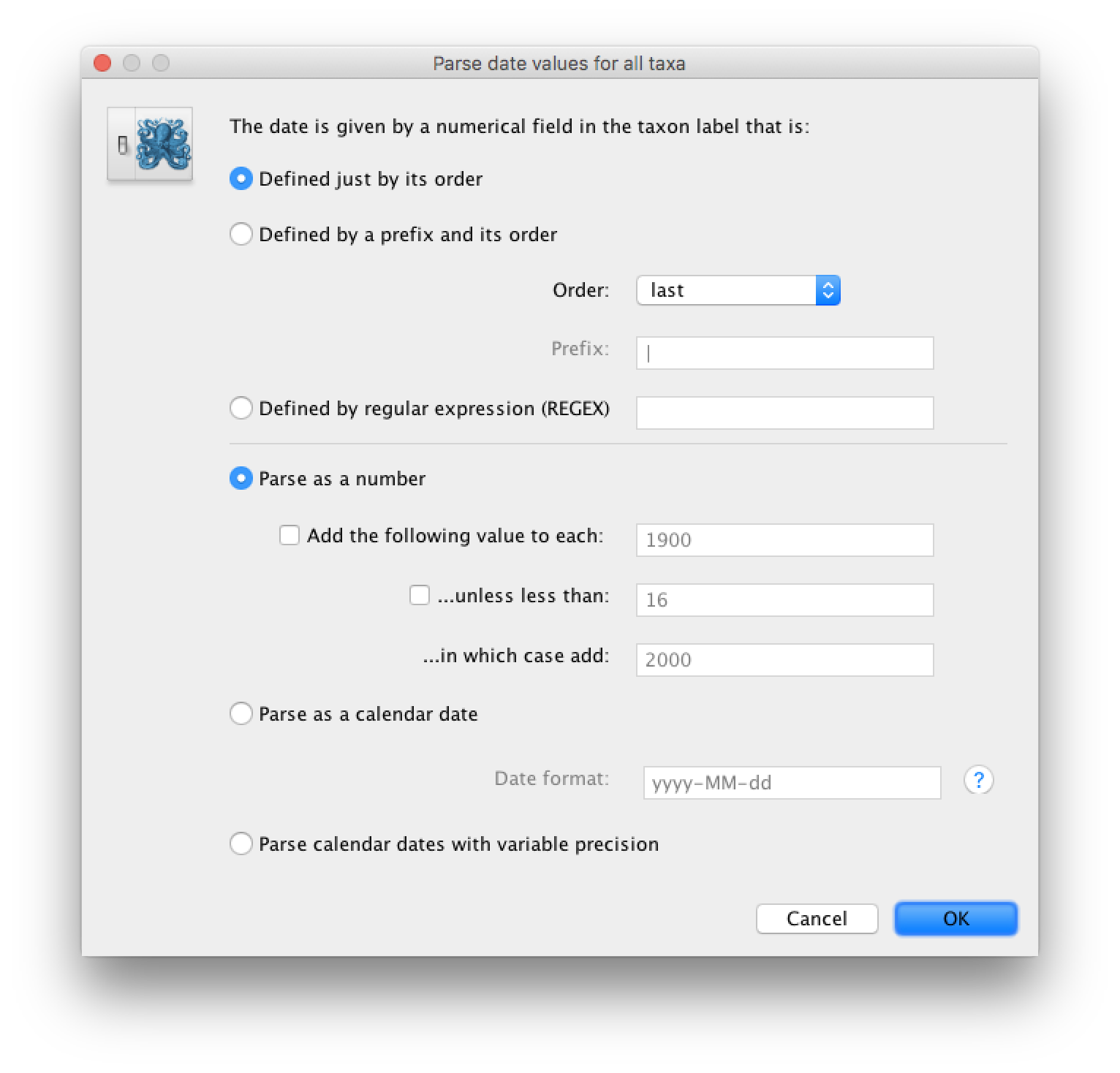
This operation attempts to guess what the dates are from information contained within the taxon names. It works by trying to find a numerical field within each name. If the taxon names contain more than one numerical field then you can specify how to find the one that corresponds to the date of sampling. See this page for details about the various options for setting dates in this panel. For the RABV sequences you can keep the default Defined just by its order and Order: last and press OK. The dates will appear in the appropriate column of the main window.
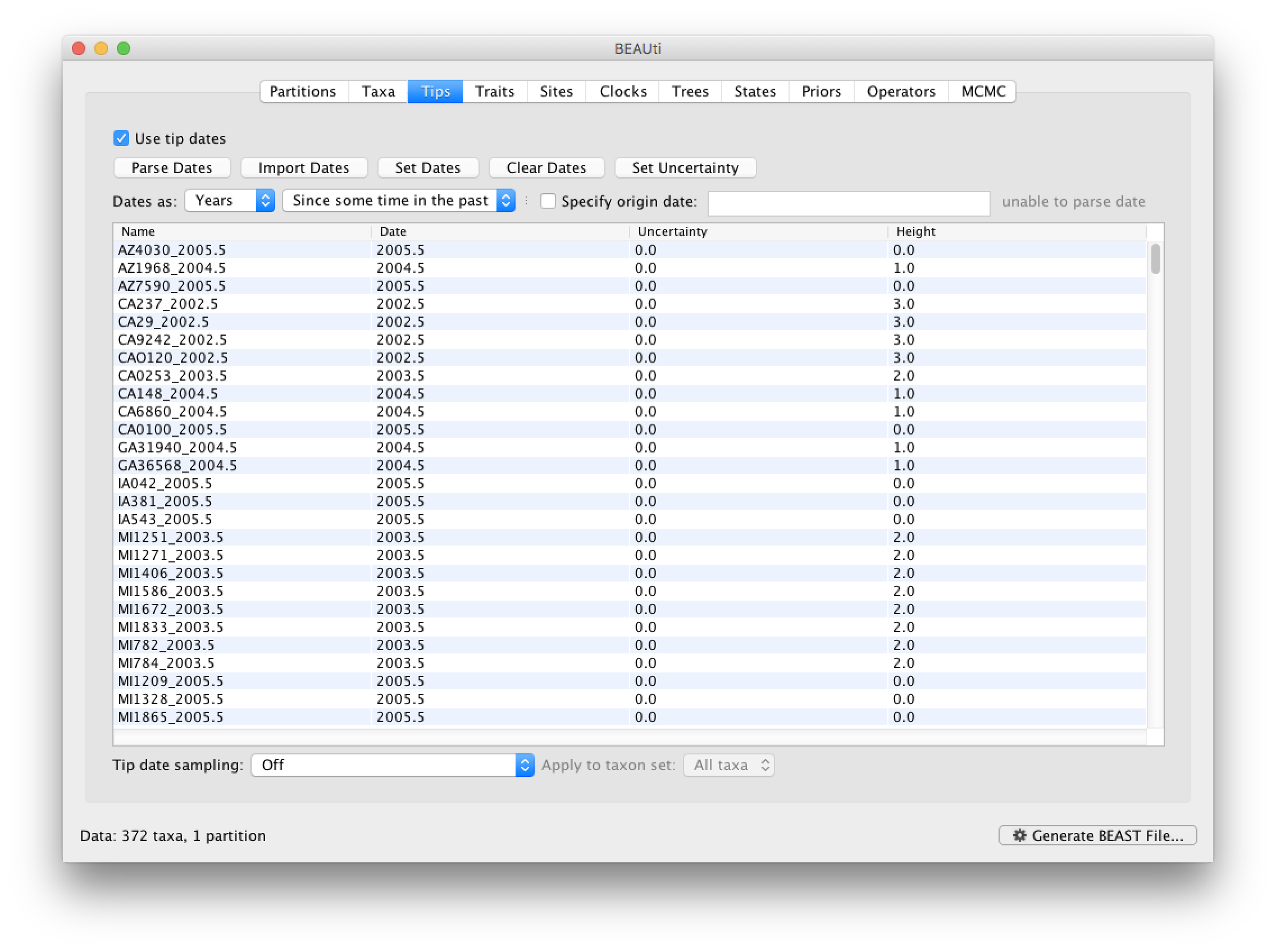
You can now check these and edit them manually as required. At the top of the window you can set the units that the dates are given in (years, months, days) and whether they are specified relative to a point in the past (as is the case for years such as 2005) or backwards in time from the present (as in the case of radiocarbon ages).
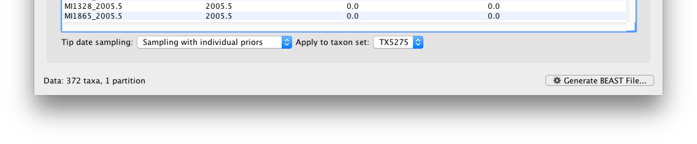
The Height column lists the ages of the tips relative to time 0 (in our case 2005.5). The Uncertainty column allows you to specify with what uncertainty the sampling time is known. If a time is only known to the year of sampling, for example, an uncertainty of 1 year can be set and the age of that tip can be integrated over the time interval of 1 year using the Tip date sampling option at the bottom left of the Tips panel. An uncertainty of one year could be specified for this RABV data set, but this uncertainty is small relative to the time scale of this evolutionary history, so we will not use it for this analysis.
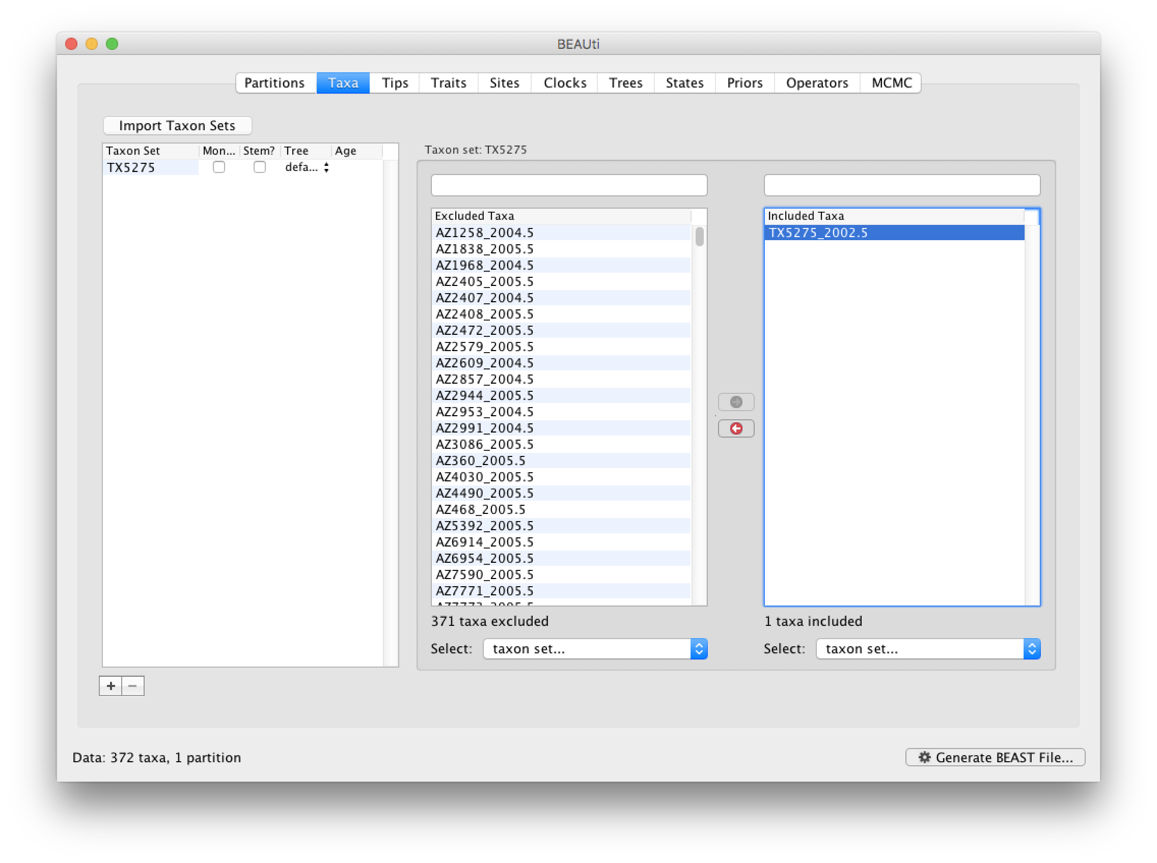
In our data set, the sampling date is unknown for one particular sequence (TX5275_2002.5, the ‘2002.5’ is simply an arbitrary date that will be used as a starting value). To appropriately accommodate the uncertainty on the age of this tip, we will instruct BEAST to integrate over a particular sampling time interval for this tip.
First, go back to the Taxa tab that we skipped, and make a taxon set for only that particular sequence. Press the small plus button at the bottom left of the panel; this creates a new taxon set. Rename it by double-clicking on the entry that appears (it will initially be called untitled1). Call it TX5275 and keep the default settings. Move TX5275_2002.5 from the Excluded Taxa window to the Included Taxa window:
Go back to the Tips tab, and in the bottom left, select the Sampling with individual priors as Tip date sampling option. Apply this to the TX5275 taxa set instead of the default All taxa option. We will set a prior on its age when we get to the Priors tab.
Specifying the trait information
The next thing to do is to click on the Traits tab at the top of the main window. A trait can be any characteristic that is inherent to the specific taxon, for example, geographical location or host species. This step will assign a specific host and geographical location to each taxa based on the trait specification for each sequence in the batRABV_hostLocation.txt file, which downloaded from here. To associate the sequences with the traits, we need to add a new trait under the Traits tab (click Add trait). This will open a new window to Create or Import Trait(s):
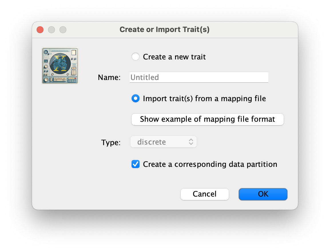
Select Import trait(s) from a mapping file (the format of such a file can be shown). Browse to and load the batRABV_hostLocation.txt tab-delimited file. Note that the host species is specified using a two-character abbreviation (e.g. Ef for Eptesicus fuscus, three characters for Lbl) as shown for this snippet of the file:
	traits	host	state
	AZ4030_2005.5	Ap	Arizona
	AZ1968_2004.5	Ef	Arizona
	AZ7590_2005.5	Ef	Arizona
	CA237_2002.5	Ef	California
	CA29_2002.5	Ef	California
	CA9242_2002.5	Ef	California
	CAO120_2002.5	Ef	California
	CA0253_2003.5	Ef	California
	CA148_2004.5	Ef	California
	CA6860_2004.5	Ef	California
	CA0100_2005.5	Ef	California
	GA31940_2004.5	Ef	Georgia
		...
	TX3545_2004.5	Tb	Texas
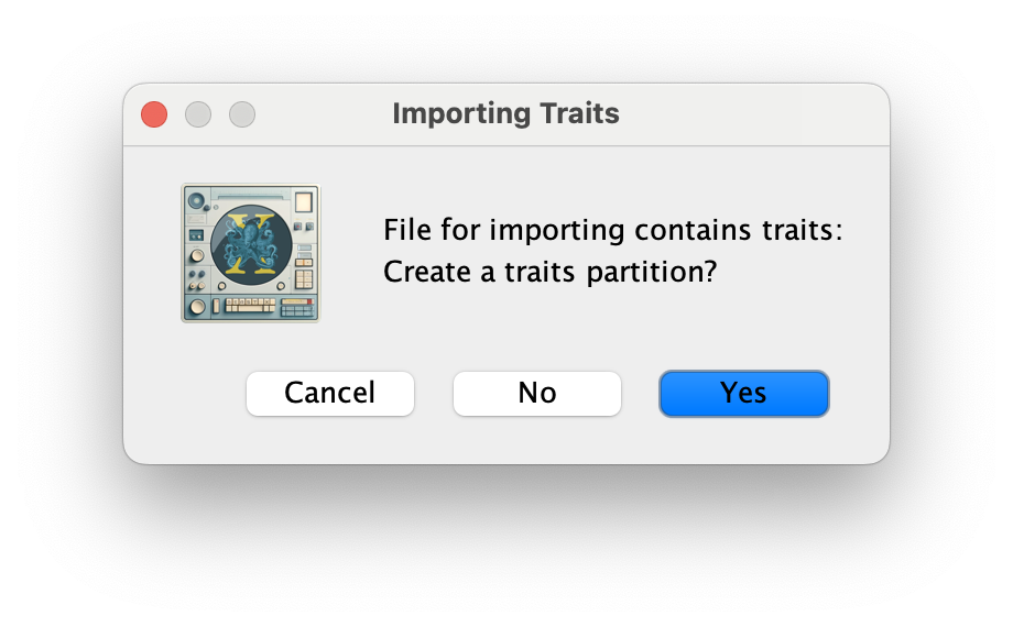
Click OK, and Yes in the following window. Then, select both the host and state traits, click on New partition for each trait and click OK.
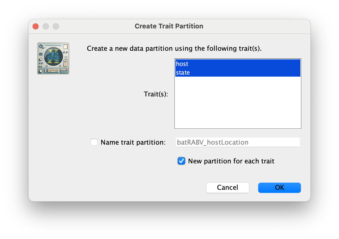
These new partitions will be shown under the Partitions tab, resulting in three partitions in the Partitions tab:
Setting the sequence and trait evolutionary models
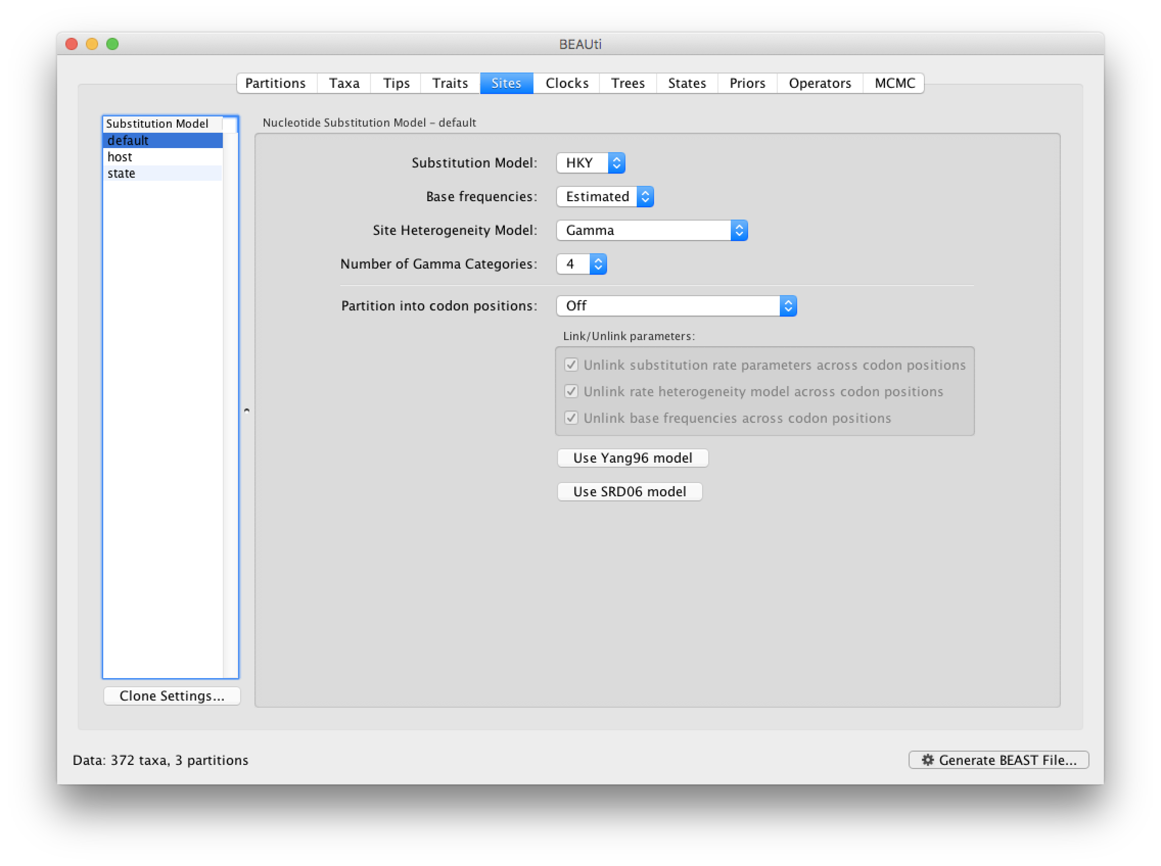
The next thing to do is to click on the Sites tab at the top of the main window. This will reveal the evolutionary model settings for BEAST. For the nucleotide model in this tutorial, keep the default HKY substitution model, set base frequencies to Empirical, and use Gamma-distributed rate variation among sites (with 4 discrete categories):
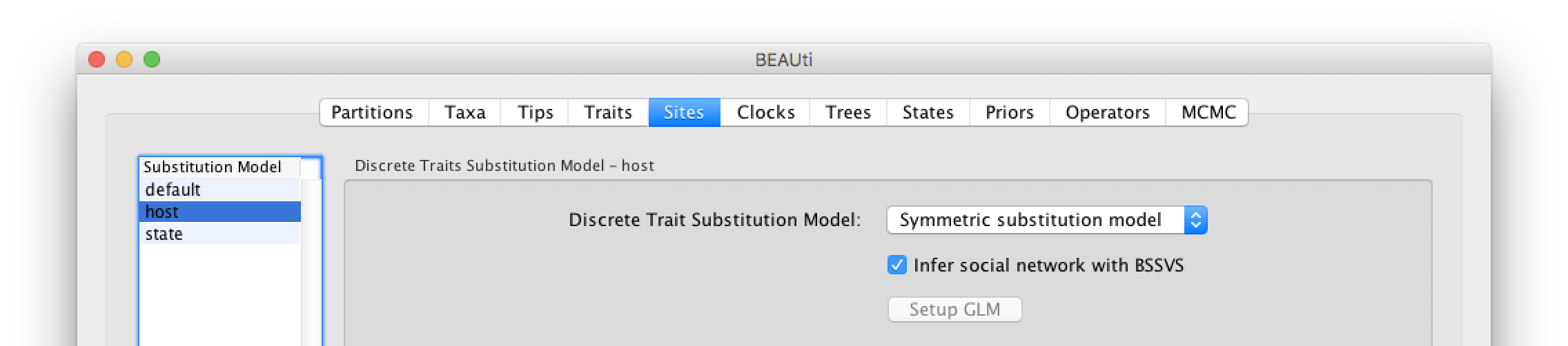
Click on ‘host’ in the Substitution model window and keep the Discrete Trait Substitution Model as Symmetric substitution model but select the option to perform BSSVS (Infer social network with BSSVS). The symmetric substitution model specifies a discrete state ancestral reconstruction using a standard continuous-time Markov chain (CTMC), in which the transition rates between locations are reversible. The alternative Asymmetric substitution model specifies a discrete state ancestral reconstruction using a nonreversible CTMC. Selecting the BSSVS option enables the Bayesian Stochastic Search Variable Selection procedure. This procedure will attempt to limit the number of rates (at least k-1, where k is the number of states) to only those that adequately explain the phylogenetic diffusion process.
Apply the same discrete diffusion model settings to the geographic state trait.
Setting the ‘molecular clock’ model
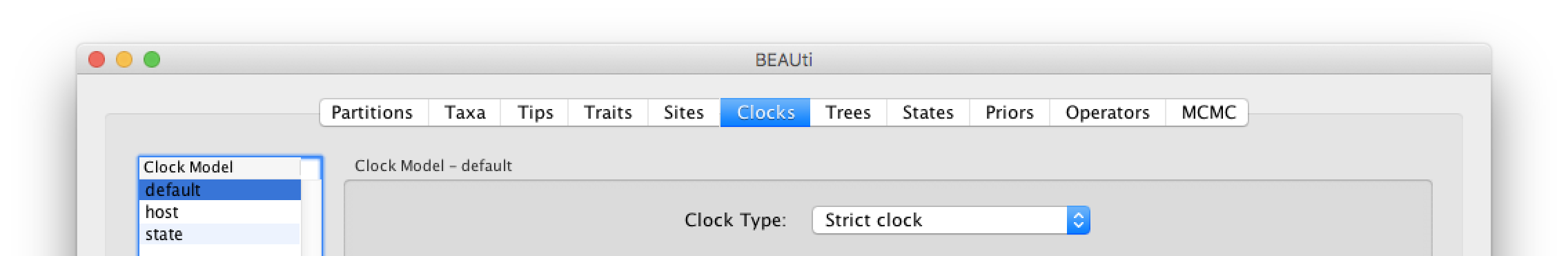
The ‘Molecular Clock Model’ options in the Clocks panel allows us to choose between a strict and a relaxed (uncorrelated lognormal or uncorrelated exponential) clock. We will perform our run using the default Strict clock model:
We can also keep default settings for overall rate scalers in the host and geographic state transition processes.
Now move on to the Trees panel.
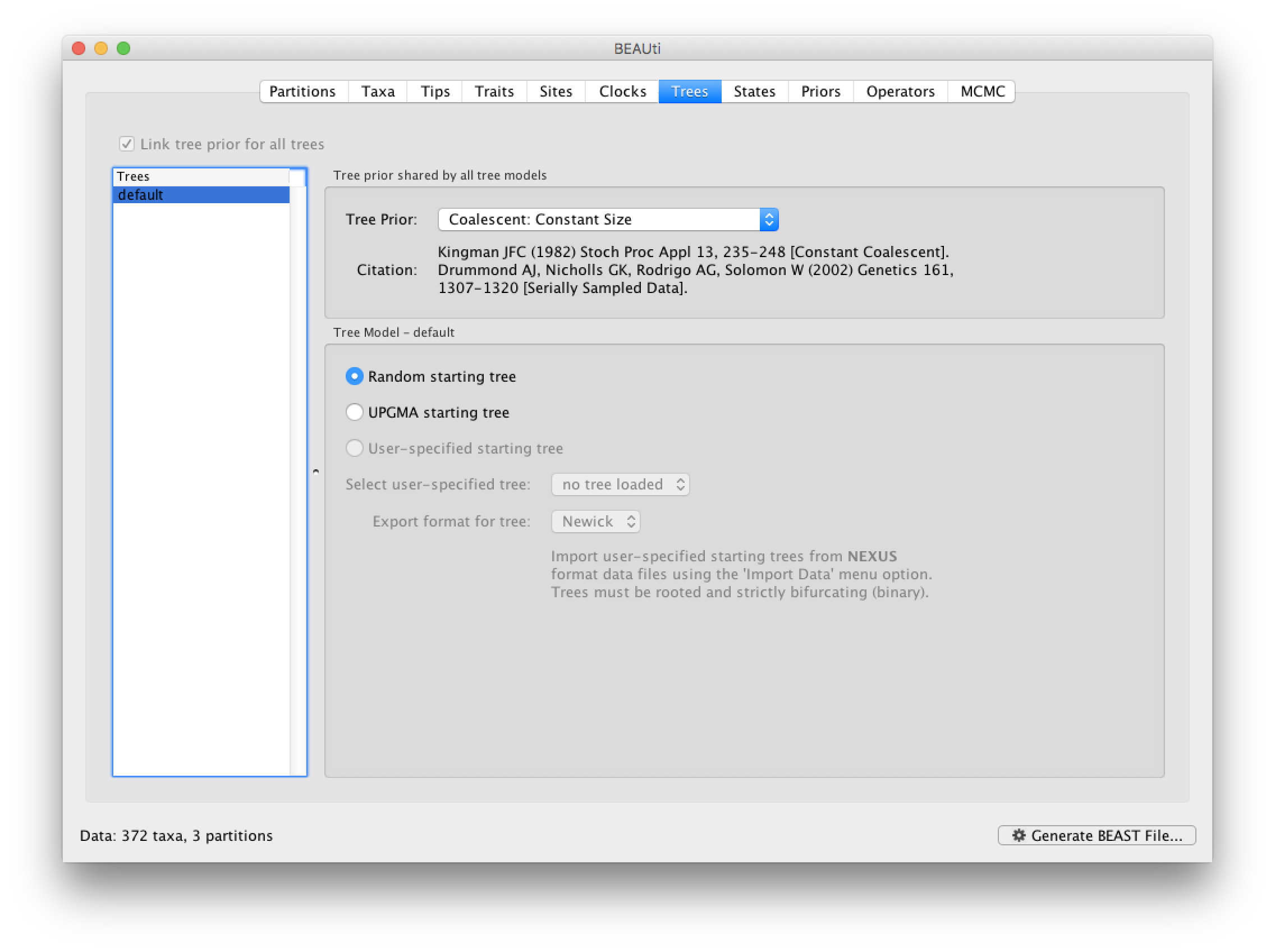
Setting the tree prior
This panel contains settings about the tree. Firstly the starting tree is specified to be a Random starting tree. The other main setting here is to specify the Tree prior which describes how the population size is expected to change over time according to a coalescent model. The default tree prior is set to a constant size coalescent prior. In this tutorial, we will keep these default settings.
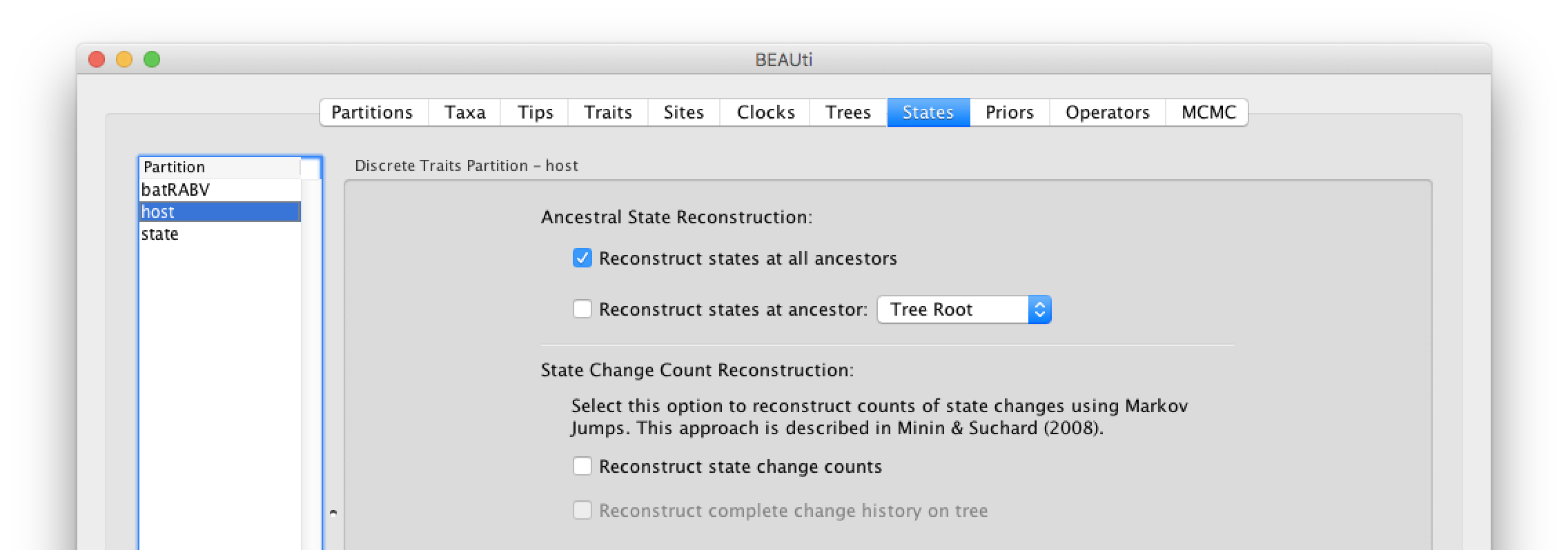
The ancestral states settings
In the States panel, check that for the host and state partition the option to Reconstruct states at all ancestors is selected (by default).
Setting up the priors
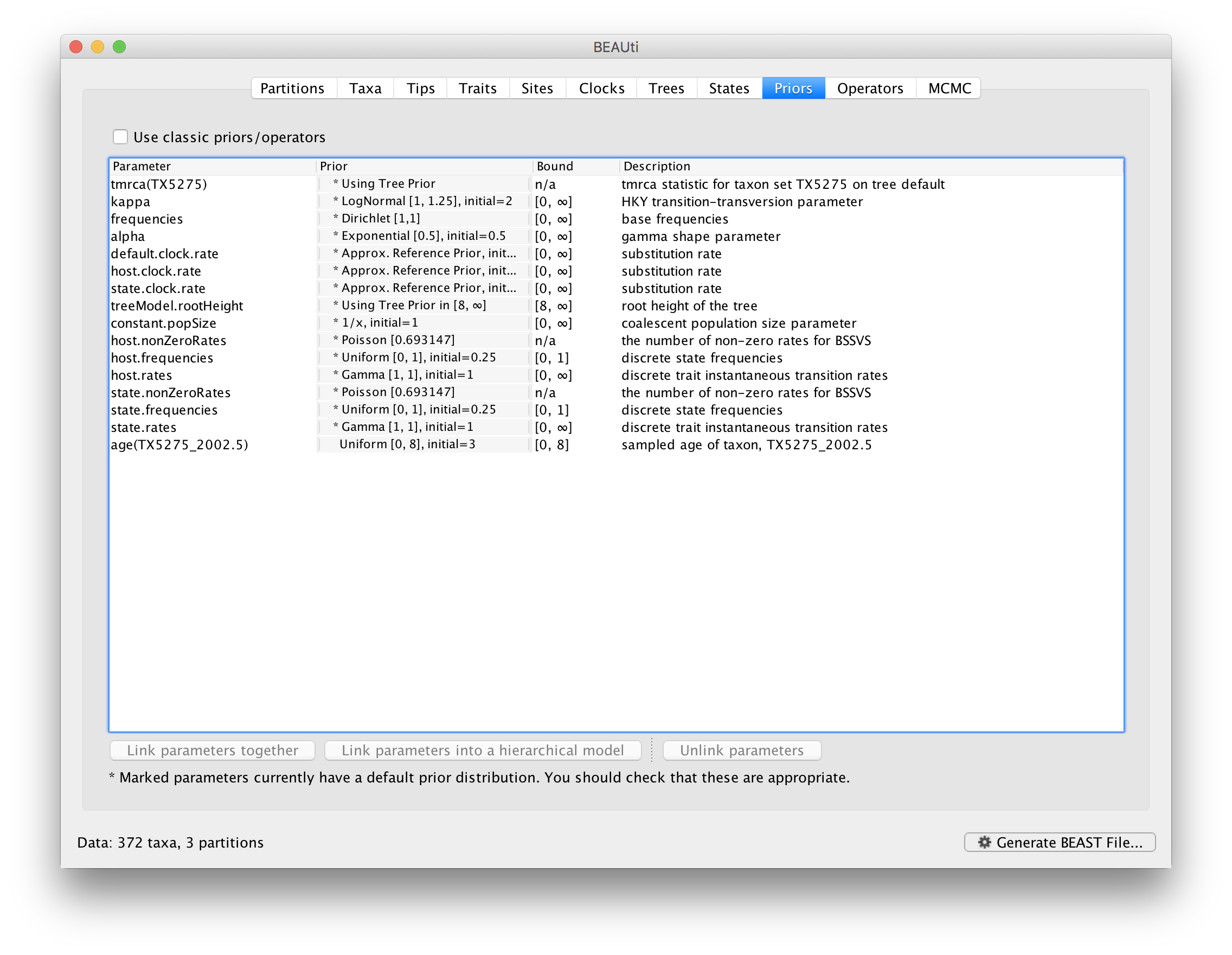
Now switch to the Priors tab. This panel has a table showing every parameter of the currently selected model and what the prior distribution is for each. A strong prior allows the user to ‘inform’ the analysis by selecting a particular distribution with a small variance. Alternatively we can select a weak (diffuse) prior to try to minimise the effect on the analysis. Note that a prior distribution must be specified for every parameter and whilst BEAUti provides default options these are not necessarily tailored to the problem and data being analyzed.
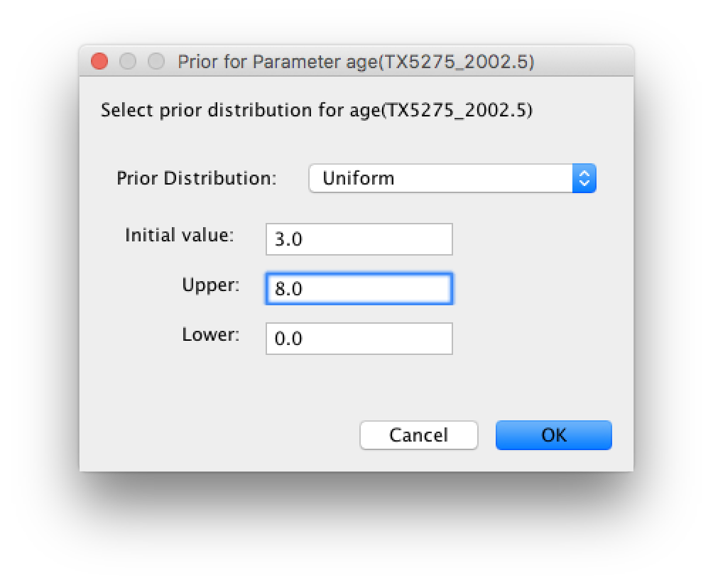
The default prior on the rate of evolution (clock.rate) is an approximation of a conditional reference prior (Approx. Reference Prior) (Ferreira and Suchard, 2008). The same is applied to the discrete host and location state rate. There is also a default uniform prior specification for the age of TX5275 (age(TX5275_2002.5) ). We will assume that the sampling time for this tip is bounded by the sampling time range for all taxa this data set, implying that it is sampled between 1997.5 and 2005.5. Click on the current uniform prior setting, set the Upper age to 8 years (reflecting the 1997.5 boundary) and click OK.
The resulting prior table will look like this:
Setting up the operators
Each parameter in the model has one or more “operators” (these are variously called moves, proposals or transition kernels by other MCMC software packages such as MrBayes and LAMARC). The operators specify how the parameters change as the MCMC runs. The Operators tab in BEAUti has a table that lists the parameters, their operators and the tuning settings for these operators:
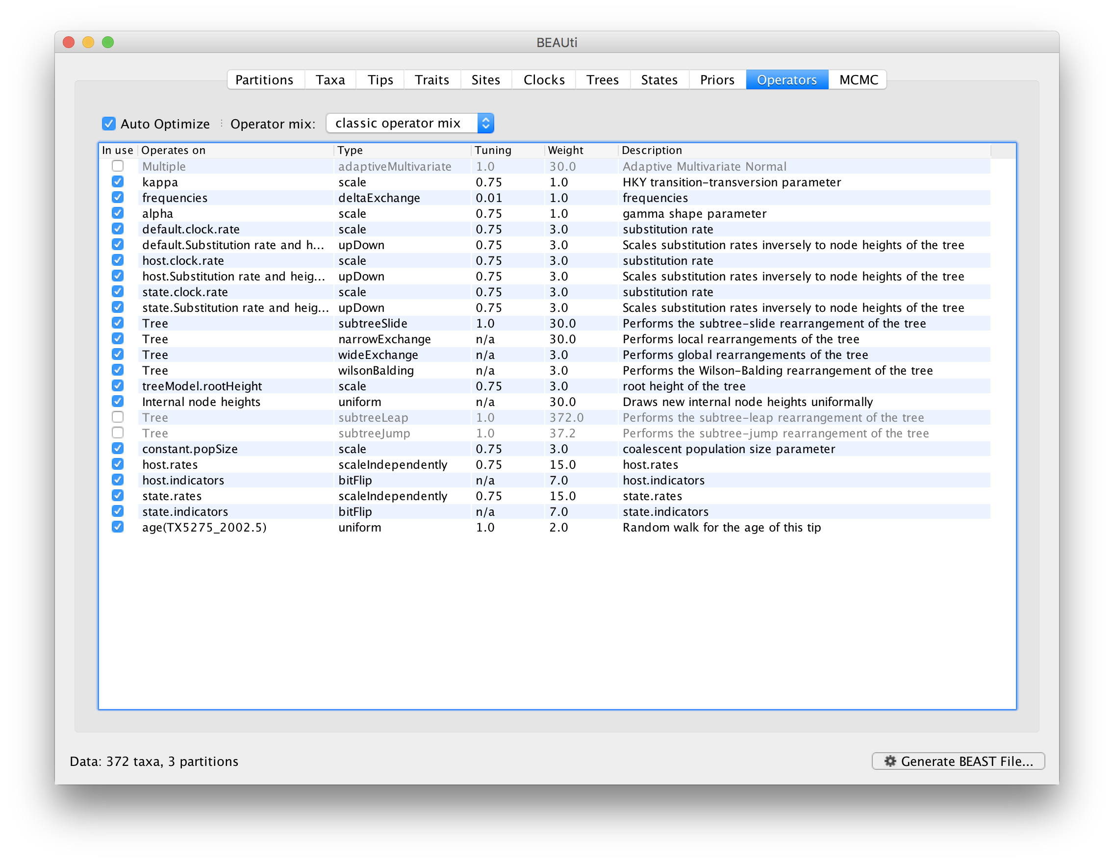
We can keep the default operator settings for the current analysis.
Setting the MCMC options
The MCMC tab in BEAUti provides settings to control the MCMC chain and the log files that get produced.
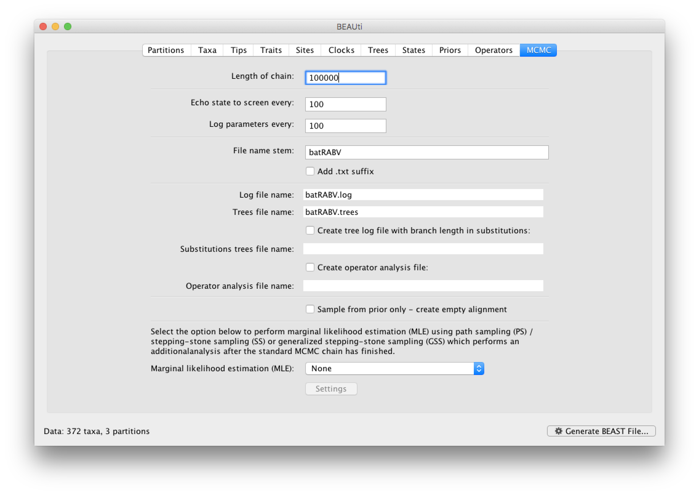
For this dataset let’s initially set the chain length to 100,000 and both the sampling frequencies to 100. The File name stem: should already be set to batRABV but you can adjust this (perhaps add more indications about the analysis).
We are now ready to create the BEAST XML file. Select Generate XML... from the File menu (or the button at the bottom of the window). BEAUti will ask you to review the prior settings one more time before saving the file (and will indicate if any are improper). Continue and choose a name for the file — it will offer the name you gave it in the MCMC panel and we usually end the filename with ‘.xml’ (although on Windows machines you may want to give the file the extension ‘.xml.txt’).
Running BEAST
Once the BEAST XML file has been created the analysis itself can be performed using BEAST.
Once BEAST has started a dialog box will appear in which you select the XML file:
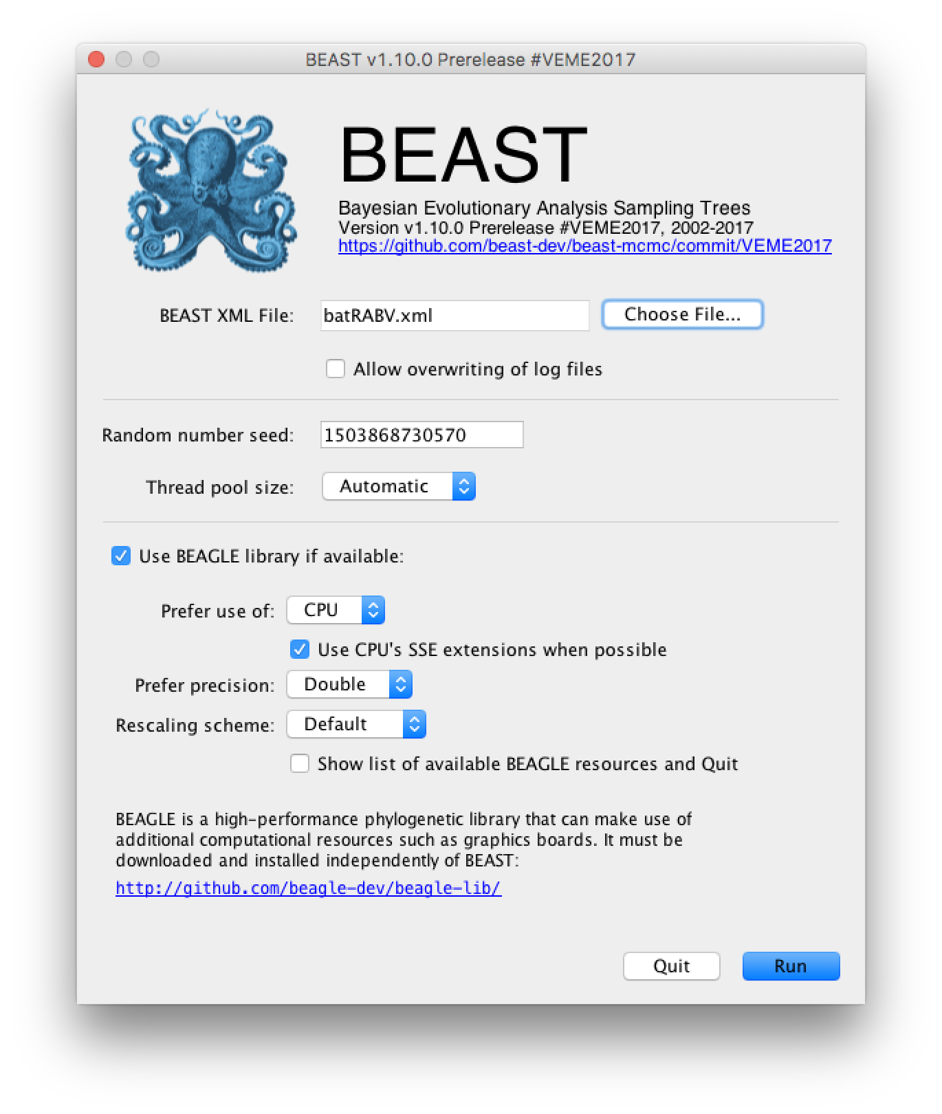
Press the Choose File... button and select the XML file you just created and press Run. The analysis will then be performed with detailed information about the progress of the run being written to the screen. When it has finished, the log file and the trees file will have been created in the same location as your XML file.
For more information about the other options in the BEAST dialog box see this page.
Analyzing the BEAST output using Tracer
To analyze the results of running BEAST we are going to use the program Tracer. The exact instructions for running Tracer differs depending on which computer you are using. Double click on the Tracer icon; once running, Tracer will look similar irrespective of which computer system it is running on.
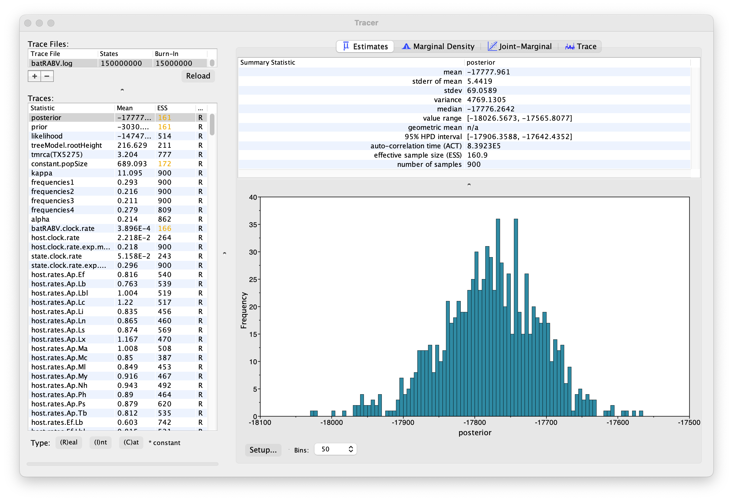
Select the Import Trace File... option from the File menu. If you have it available, select the log file that you created in the previous section (batRABV.log). Alternatively, drag and drop your log file into the Tracer window. The file will load and you will be presented with a window similar to the one below. Remember that MCMC is a stochastic algorithm so the actual numbers will not be exactly the same.
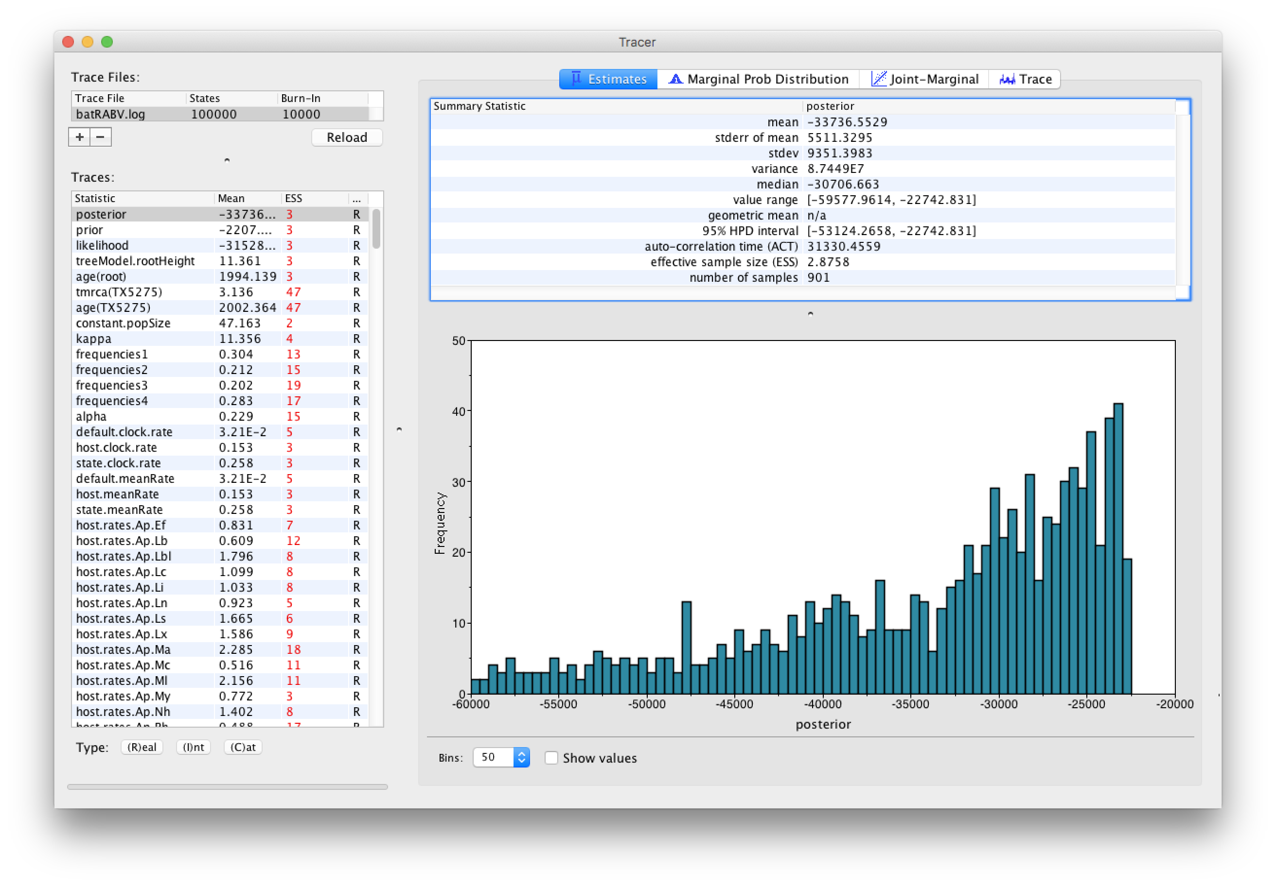
On the left hand side is the name of the log file loaded and the traces that it contains. There are traces for the posterior (this is the log of the product of the tree likelihood and the prior probabilities), and the continuous parameters. Selecting a trace on the left brings up analyses for this trace on the right hand side depending on tab that is selected. When first opened, the ‘posterior’ trace is selected and various statistics of this trace are shown under the Estimates tab.
Note that the effective sample sizes (ESSs) for all the traces are small. Select the Trace panel from the top of the window and inspecting the traces of the various parameters. You will see that the chain is still in the burn-in phase (the posterior values are still increasing over the entire chain), and this run does not allow us to summarize marginal posterior probability distributions for the parameters.
The simple response to this situation is that we need to run the chain for longer. We have provided the results of a very long run — 150 million steps, sampling every 150,000th step, resulting in 1,000 samples. In this case, the MCMC run has reached stationarity, and almost all parameter traces still show satisfactory ESSs.
You can load the long run log file (batRABV.log) into the same Tracer window for comparison to the short run. This gives this:
We can continue to summarize the annotated phylogeographic tree inferred with the BSSVS procedure and estimate the most significant rates of diffusion. If you are only interested in summarizing the Bayes Factor rates from the BSSVS analysis and not in summarizing the tree from your run, jump to the last section of this tutorial entitled Visualizing tree and calculating Bayes factor support for rates using SPREAD4.
Summarizing and visualizing the trees
At this point you can summarize the sampled trees using the TreeAnnotator utility and then visualize the resulting tree using the FigTree application.
Visualizing MCC trees and calculating Bayes factor support for rates using SPREAD 4
SPREAD4, i.e. Spatial Phylogenetic Reconstruction of EvolutionAry Dynamics version 4, is a software to visualize the output from Bayesian phylogeographic analysis and constitutes a user-friendly application to analyze and visualize reconstructions resulting from Bayesian inference of sequence and trait evolutionary processes. SPREAD 4 allows to visualise spatial reconstructions on custom maps and is run entirely online in browsers such as Firefox, Safari and Chrome.
Some of the functions that relate to the discrete phylogeographic analysis include visualizing location-annotated MCC trees and identification of well-supported rates using a Bayes Factor test. The latter option takes as input the rate matrix file (batRABV.state.rates.log for location states and batRABV.host.rates.log for host states) generated under the analysis using the Bayesian Stochastic Search Variable Selection (BSSVS) procedure. This test aims at identifying frequently invoked rates to explain the diffusion process and, in case of locations, visualize them on a circle and on a globe or a map, which needs to be provided to SPREAD4.
To get started with SPREAD 4,follow the instructions here.
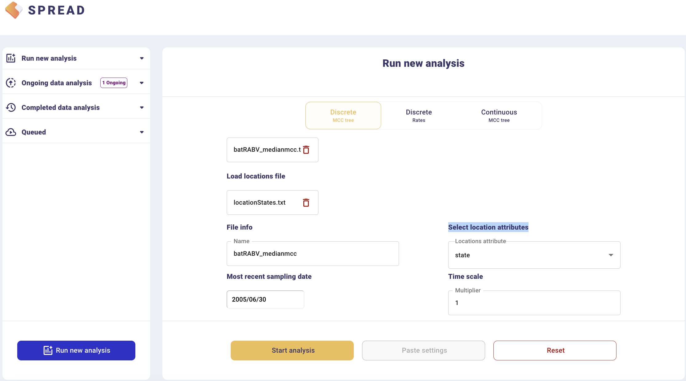
To visualize an MCC tree, click on Run new analysis and select the Discrete MCC tree tab. Load the MCC tree and coordinates in the ‘locationStates.txt’ file, which should look like this:
	Arizona		33.7712	-111.3877
	California	36.17	-119.7462
	Georgia		32.9866	-83.6487
	Iowa		42.0046	-93.214
	Michigan	43.3504	-84.5603
	NewJersey	40.314  -74.5089
	Virginia	37.43157    -78.656895
	Washington	47.3917	-121.5708
	Florida		27.8333	-81.717
	Tennessee	35.7449	-86.7489
	Texas		31.106	-97.6475
	Idaho		44.2394	-114.5103
	Indiana		39.8647	-86.2604
	Mississippi	32.7673	-89.6812
The coordinates can be downloaded here.
This will load the locations and their lat/long coordinates. Set the most recent sampling date (2005.5) to 2006/06/30, and click Start analysis.
The analysis will first appear in the left-side tab Queued and then in the Completed Data Analysis.
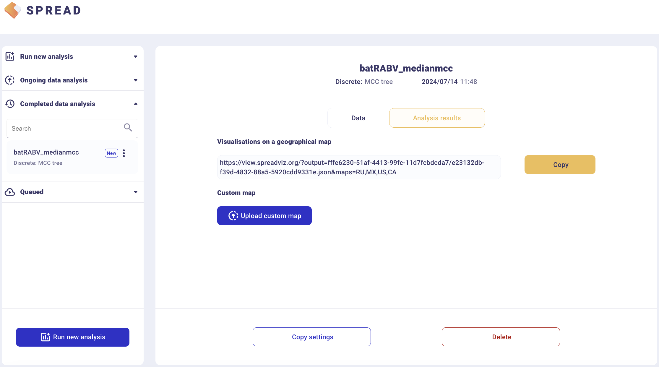
There is an option to load a custom map of the United States in GeoJSON format. Such a map is provided amongst the data files — gz_2010_us_040_00_500k.json. However, a default map is provided to visualize the results. Click Copy and open the link in a new browser tab/window.
To summarise Bayes factor support for rates, select the Discrete Rates tab. Load the output BEAST file containing the spatial rates and rate indicators (batRABV.state.rates.log) and the coordinates in the locationStates.txt file, and set an appropriate burn-in level. Click, Start analysis.
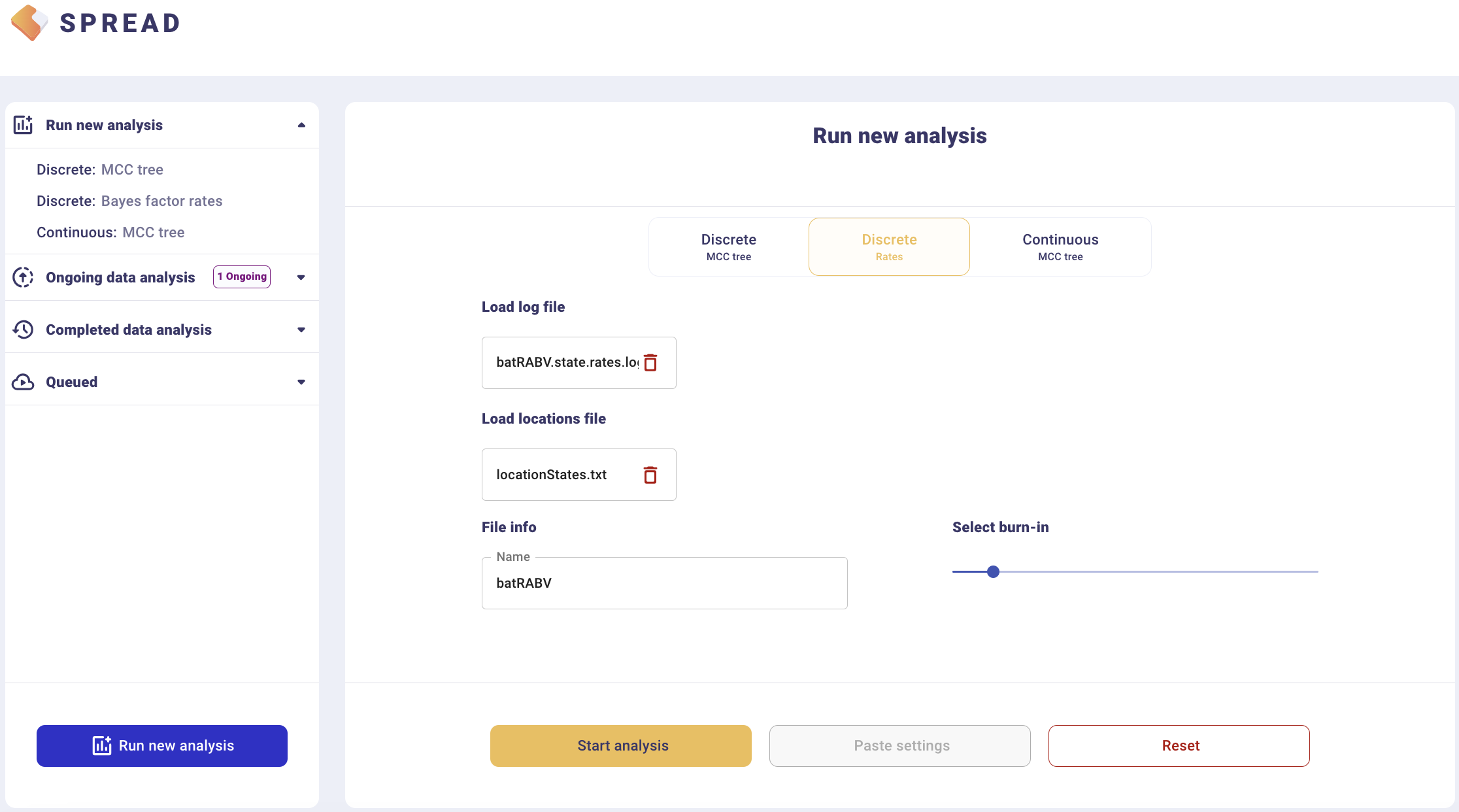
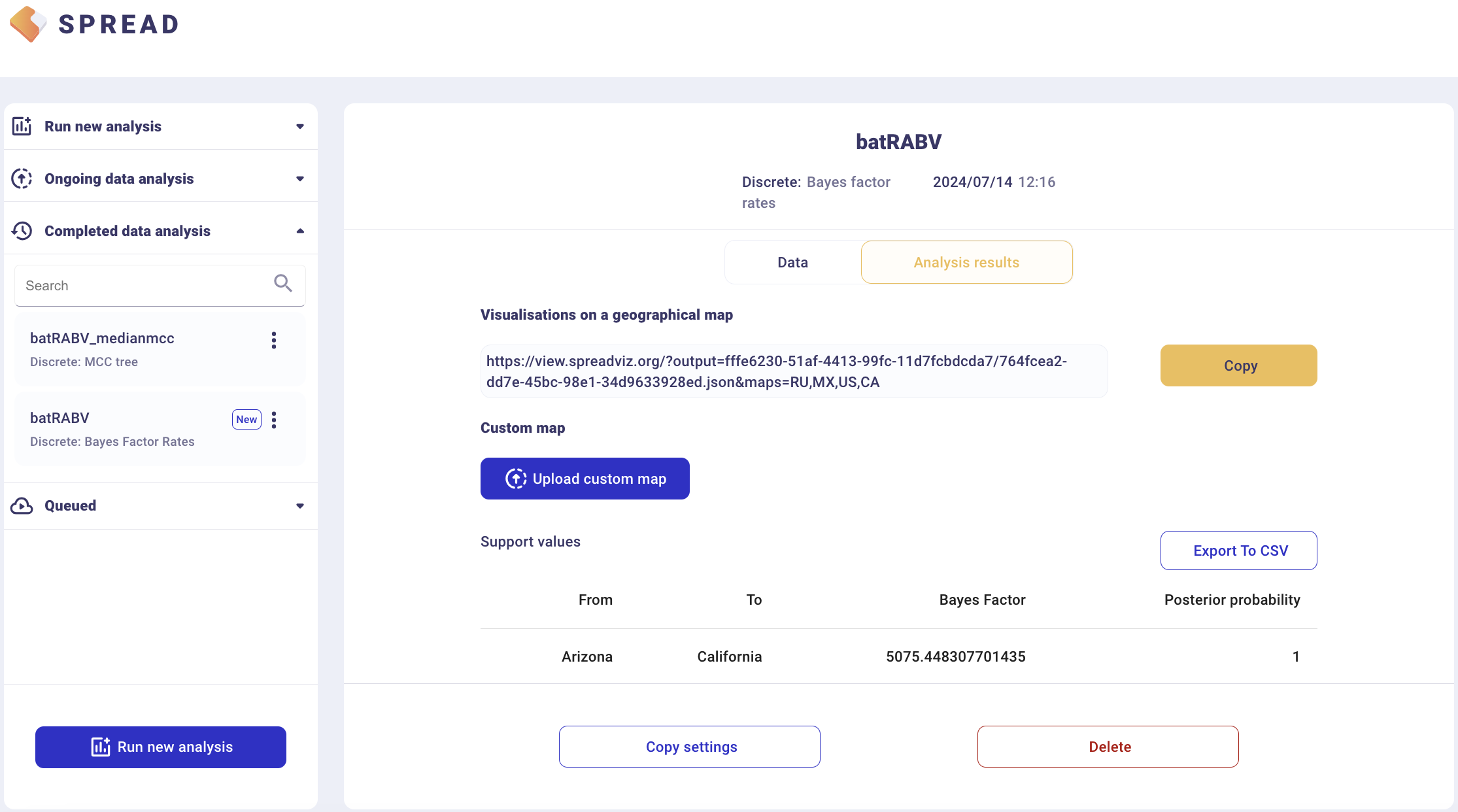
The analysis will first appear in the left-side tab Queued and then in the Completed Data Analysis.
There is an option to load a custom map of the United States in GeoJSON format. Such a map is provided amongst the data files — gz_2010_us_040_00_500k.json. However, a default map is provided to visualize the results. Click Copy and open the link in a new browser tab/window. Note that a comma-separated value file with a ‘.csv’ extension containing the actual Bayes Factor values can be downloaded by clicking Export to CSV.
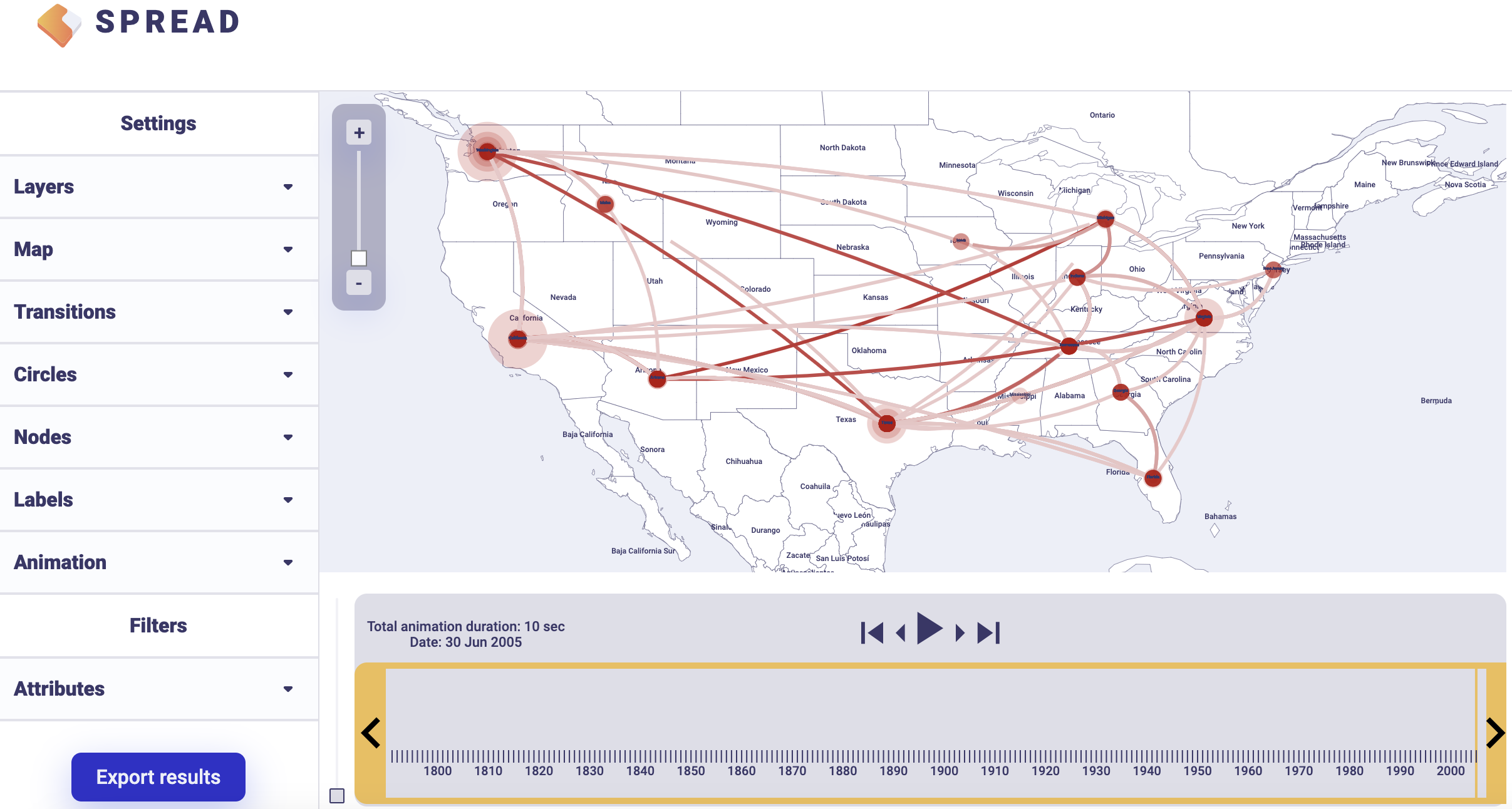
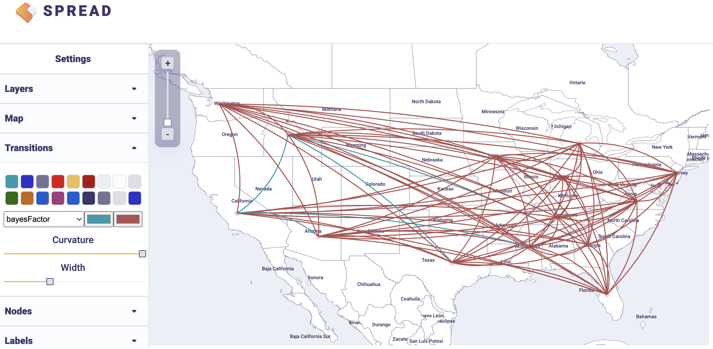
An example visualisation can be found below. Note that the visual aspects of the lines representing the rates can be modified and that the lines can also be filtered by a cut-off (under Filters and Attributes).
EXERCISE 2: Identifying predictors for the host switching process
Background
This exercise builds on the previous analysis and aims at testing the factors that drive the host transitioning process for bat rabies viruses in North America. The original analyses resorted a population genetic approach and post hoc statistical procedures to test such predictors (Streicker et al., 2010); here we adopt an extension of the discrete diffusion model as applied by Faria et al. (2013). This extension parameterizes the CTMC matrix as a generalized linear model (GLM), in which log CTMC rates are a log linear function of several potential predictors (most of the detail on the model can be found in Lemey et al., 2014). We use the predictors originally proposed by Streicker et al. (2010): host phylogenetic distance (based on host mitochondrial DNA), geographic range overlap, roost structure overlap, and foraging niche overlap as approximated using three morphological measurements: wing aspect ratio, wing loading and body length, which are associated with foraging behavior in bats. We also consider sequence sample sizes, which can bias ancestral reconstructions, for both the ‘donor’ and ‘recipient’ host as additional predictors (cfr. Lemey et al., 2014).
GLM-diffusion model specification
Repeat the first BEAUti steps up to setting the setting the sequence and trait evolutionary models. In case the BEAUti session from the previous exercise has not been closed yet, simply go back to the Sites panel. For the ‘host’ trait under Substitution Model, select Generalized Linear Model:
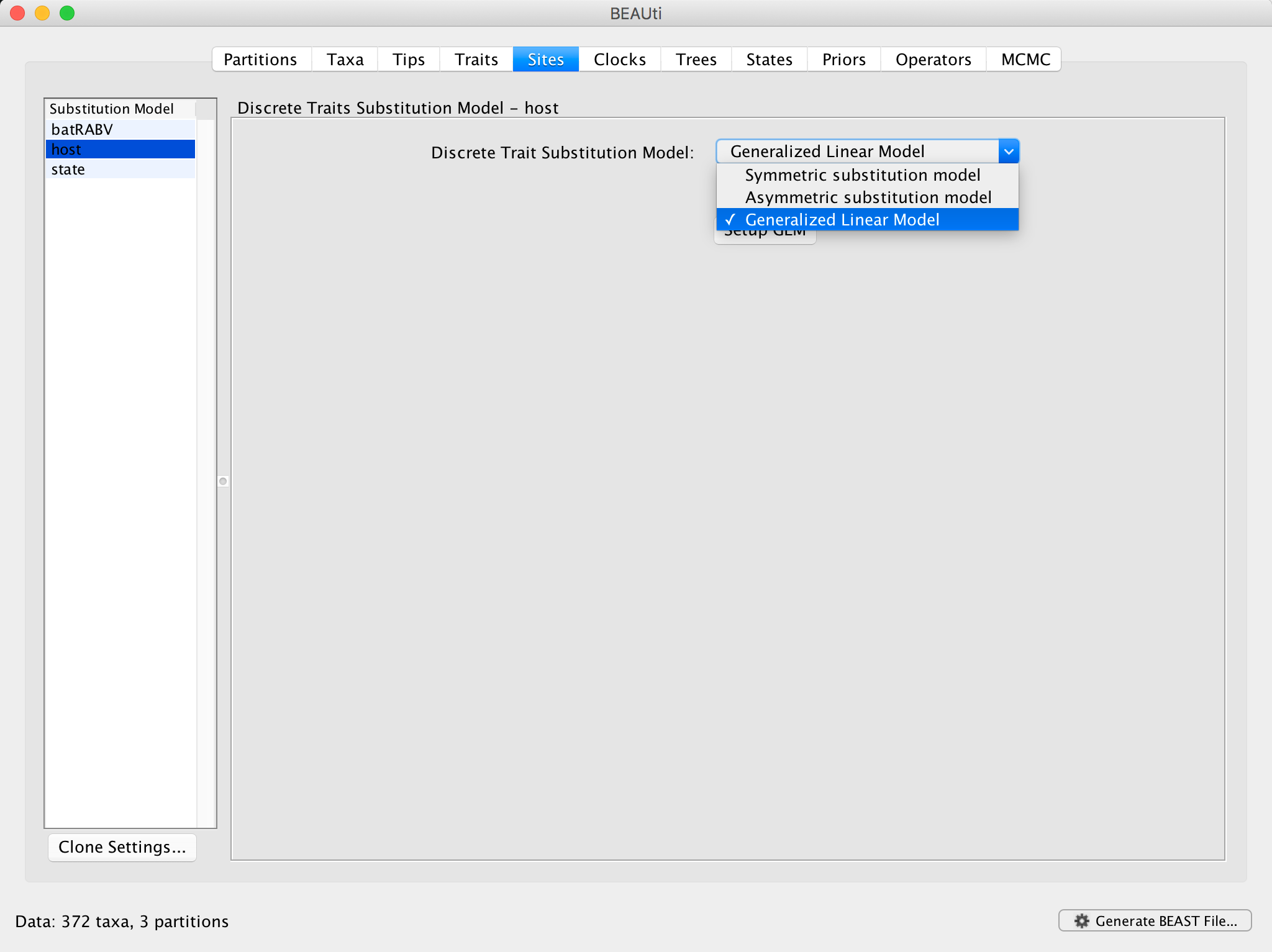
Click on Setup GLM and a new window will pop up:
This window allows specifying a set of GLM predictors or covariates by importing them through Import Predictors.... All predictors can be downloaded as a zipped folder here or as individual files linked below.
Start by loading the distance matrix between bat rabies hosts based on mitochondrial gene distances (hostDistances.csv). This is a csv file with the following content (the two-character labels represent the bat species):
	,Ap,Ef,Lb,Lbl,Lc,Li,Ln,Ls,Lx,Ma,Mc,Ml,My,Nh,Ph,Ps,Tb
	Ap,0,0.745,0.878,0.8,0.71,0.86,0.711,0.916,0.788,0.794,0.717,0.736,0.78,0.74,0.596,0.67,0.923
	Ef,0.745,0,0.971,0.893,0.803,0.953,0.586,1.009,0.881,0.887,0.81,0.829,0.873,0.615,0.689,0.763,1.016
	Lb,0.878,0.971,0,0.316,0.546,0.696,0.937,0.118,0.624,0.944,0.867,0.886,0.93,0.966,0.746,0.82,0.839
	Lbl,0.8,0.893,0.316,0,0.468,0.618,0.859,0.354,0.546,0.866,0.789,0.808,0.852,0.888,0.668,0.742,0.761
	Lc,0.71,0.803,0.546,0.468,0,0.65,0.769,0.584,0.578,0.776,0.699,0.718,0.762,0.798,0.578,0.652,0.671
	Li,0.86,0.953,0.696,0.618,0.65,0,0.919,0.734,0.357,0.926,0.849,0.868,0.912,0.948,0.728,0.802,0.821
	Ln,0.711,0.586,0.937,0.859,0.769,0.919,0,0.975,0.847,0.853,0.776,0.795,0.839,0.531,0.655,0.729,0.982
	Ls,0.916,1.009,0.118,0.354,0.584,0.734,0.975,0,0.662,0.982,0.905,0.924,0.968,1.004,0.784,0.858,0.877
	Lx,0.788,0.881,0.624,0.546,0.578,0.357,0.847,0.662,0,0.854,0.777,0.796,0.84,0.876,0.656,0.73,0.749
	Ma,0.794,0.887,0.944,0.866,0.776,0.926,0.853,0.982,0.854,0,0.273,0.292,0.196,0.882,0.576,0.65,0.989
	Mc,0.717,0.81,0.867,0.789,0.699,0.849,0.776,0.905,0.777,0.273,0,0.139,0.259,0.805,0.499,0.573,0.912
	Ml,0.736,0.829,0.886,0.808,0.718,0.868,0.795,0.924,0.796,0.292,0.139,0,0.278,0.824,0.518,0.592,0.931
	My,0.78,0.873,0.93,0.852,0.762,0.912,0.839,0.968,0.84,0.196,0.259,0.278,0,0.868,0.562,0.636,0.975
	Nh,0.74,0.615,0.966,0.888,0.798,0.948,0.531,1.004,0.876,0.882,0.805,0.824,0.868,0,0.684,0.758,1.011
	Ph,0.596,0.689,0.746,0.668,0.578,0.728,0.655,0.784,0.656,0.576,0.499,0.518,0.562,0.684,0,0.434,0.791
	Ps,0.67,0.763,0.82,0.742,0.652,0.802,0.729,0.858,0.73,0.65,0.573,0.592,0.636,0.758,0.434,0,0.865
	Tb,0.923,1.016,0.839,0.761,0.671,0.821,0.982,0.877,0.749,0.989,0.912,0.931,0.975,1.011,0.791,0.865,0
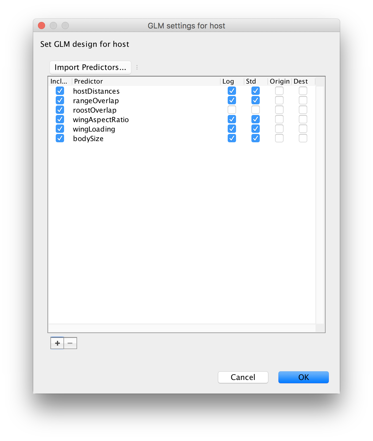
Note that by default, the values in the distance matrix are selected to be log-transformed and standardised. This is because the GLM-diffusion model parameterizes the log of the CTMC rates as a log linear function of the predictor and we grant the same variance to the predictors a priori. Repeat this procedure for range overlap (rangeOverlap.csv), roost structure overlap (roostOverlap.csv), differences in wing aspect ratio (wingAspectRatio.csv), differences in wing loading (wingLoading.csv) and differences in body size (bodySize.csv).
Note that the roost structure overlap values are ‘1’ or ‘0’ indicating whether two bat species share or not a roost structure. We will not log-transform and standardize these values (by unselecting both option) so that ‘1’ in log-space specifies an additional effect on the log transition rates for species that share a roost structure. These rates will be estimated higher or lower than the rates for species that do not share a roost structure, depending on whether the associated GLM coefficient will be estimated as positive or negative respectively in log space. After loading all predictors and unselecting the default transformations for roost structure overlap, the GLM setting for host window should look like this:
Proceed with the next steps as in the previous exercise. Note that in the Priors panel, a normal prior with mean 0 and a standard deviation of 2 is specified on the log GLM coefficients (‘host.coefficients’). We can again set up a short test run (e.g. 100,000 MCMC iterations), but proceed with diagnosing and summarising a long run. You can download the output of an MCMC analysis that has been run for 100 million iterations sampled every 50,000 generations here.
Analyzing the GLM-diffusion model output
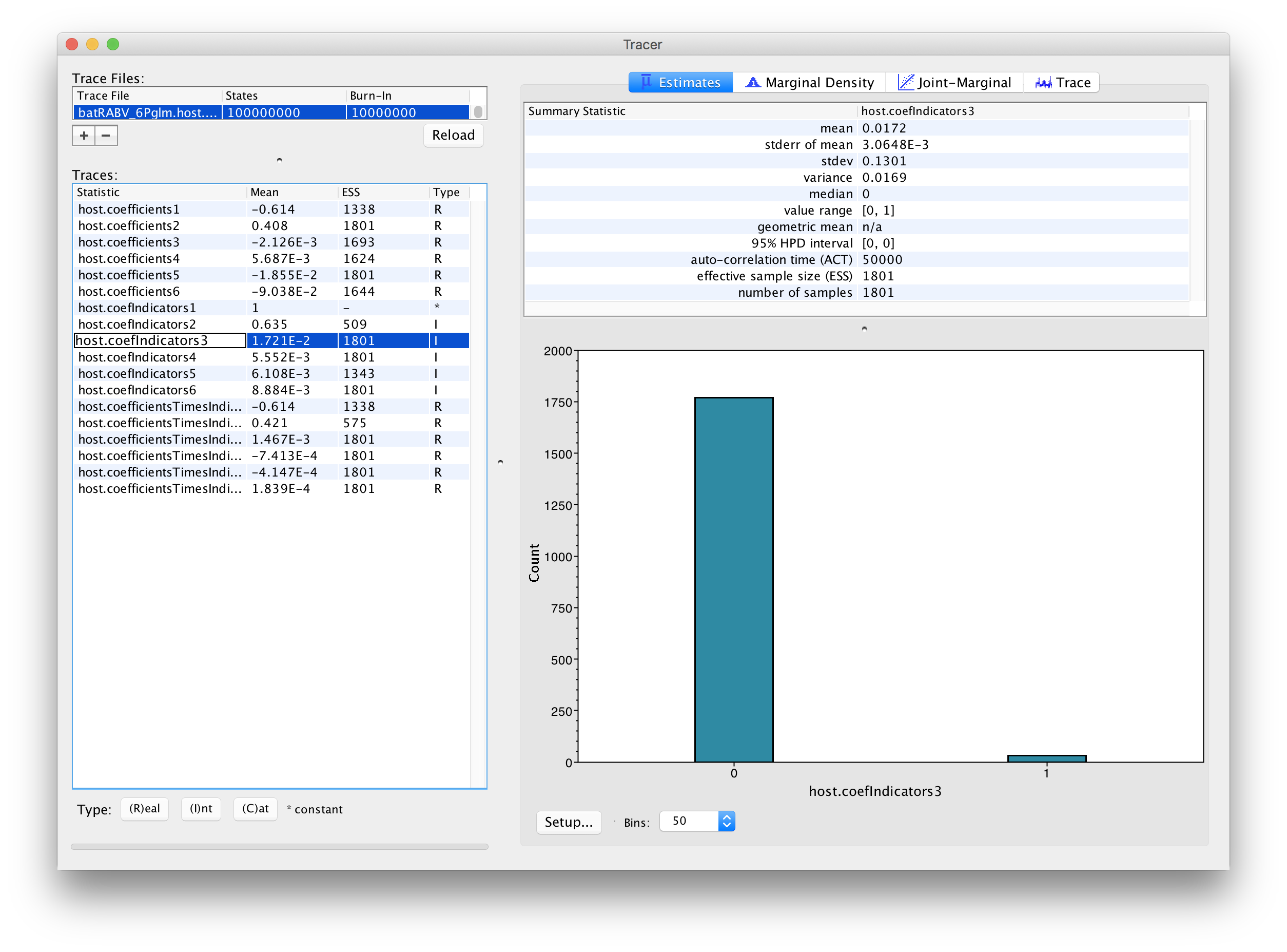
The parameters of interest in this analysis are the indicators associated with the predictors (‘host.coefIndicators1’ to ‘host.coefIndicators6’) and the coefficient parameters or effect sizes (‘host.coefficients1’ to ‘host.coefficients6’). Upon loading the log file (‘batRABV_6Pglm.host.glm.log’), the mean of an indicator provides an estimate for the inclusion probability of that indicator. In this case, the mean indicator for ‘host.coefficients1’, which represents the genetic distances between hosts, is 1 implying that this predictor is always included in the model. The second highest inclusion probability is associated with range overlap (‘host.coefficients2’) while the remaining predictors are all associated with very low inclusion probabilities.
In order to assess the evidence provided by the data for a predictor inclusion, we need to take into account the prior probability for inclusion. By default, BEAUti specifies Bernoulli prior probability distributions on these indicators with a small prior probability on each predictor’s inclusion, that is a 50% prior probability on no predictors being included, in this case:
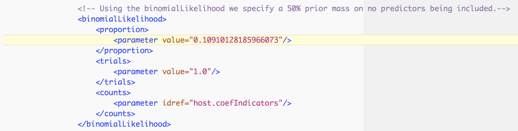
Based on both prior and posterior inclusion probabilities, we can calculate formal inclusion support in the form of Bayes Factors as these can be expressed as the ratio of the posterior odds over the prior odds for predictor inclusion. For an inclusion probability of 1, the Bayes factor is estimated as +infinity. In this case, it would be better to express the Bayes factor as being larger than X, where X would be the Bayes factor value if one sample had and indicator = 1. For range overlap, the posterior odds is 0.612/(1-0.612) = 1.577 while the prior odds is 0.109/(1-0.109) = 0.122; this results in a Bayes factor of about 13. All other predictors have posterior inclusion probabilities smaller than their prior inclusion probabilities, so they will have Bayes factors < 1.
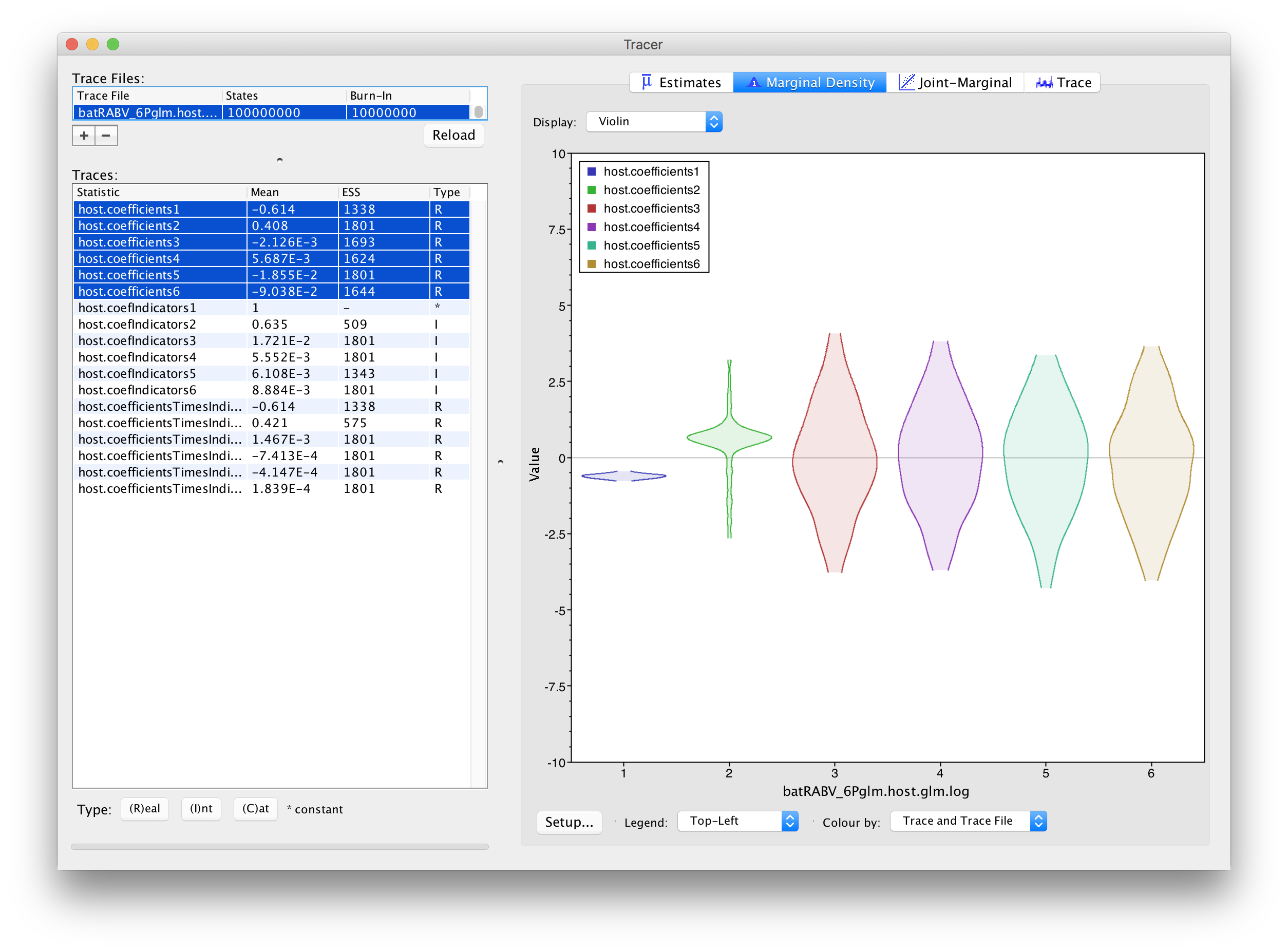
In order to assess the size of the contribution of predictors, we can use the estimates of the coefficients in log space. However, it is important to keep in mind that the estimates are critically dependent on the corresponding indicator value. If the indicator is 1, than the predictor is included in the model and the coefficient will be informed by the data (the predictor and the discrete states). If the indicator is 0, the predictor is not included and the coefficient value will be sampled from the prior. This is why posterior estimates of coefficients with very small inclusion probability will resemble the prior distribution (a normal distribution centered on 0 with a standard deviation of 2), as is the case for roost structure overlap (‘host.coefIndicators3’), differences in wing aspect ratio (‘host.coefIndicators4’), differences in wing loading (‘host.coefIndicators5’) and differences in body size (‘host.coefIndicators6’). This is demonstrated by the violin plots for these coefficients in Tracer:
This complicates the interpretation of coefficient estimates for predictors with intermediate inclusion probability (e.g., ‘host.coefIndicators2’ for range overlap). This is why applications have resorted to reporting the conditional effect size, that is the effect size when the predictors in included in the model (indicator = 1). In other words, this can be obtained by only summarising the coefficient estimates based on the samples for which the corresponding indicator values are 1. Alternatively, the predictor-specific product of the coefficient and indicator for all the samples can be summarised (these are logged as a statistic: host.coefficientsTimesIndicators1 to host.coefficientsTimesIndicators6). The violin plots fot these statistics in Tracer look as follows:
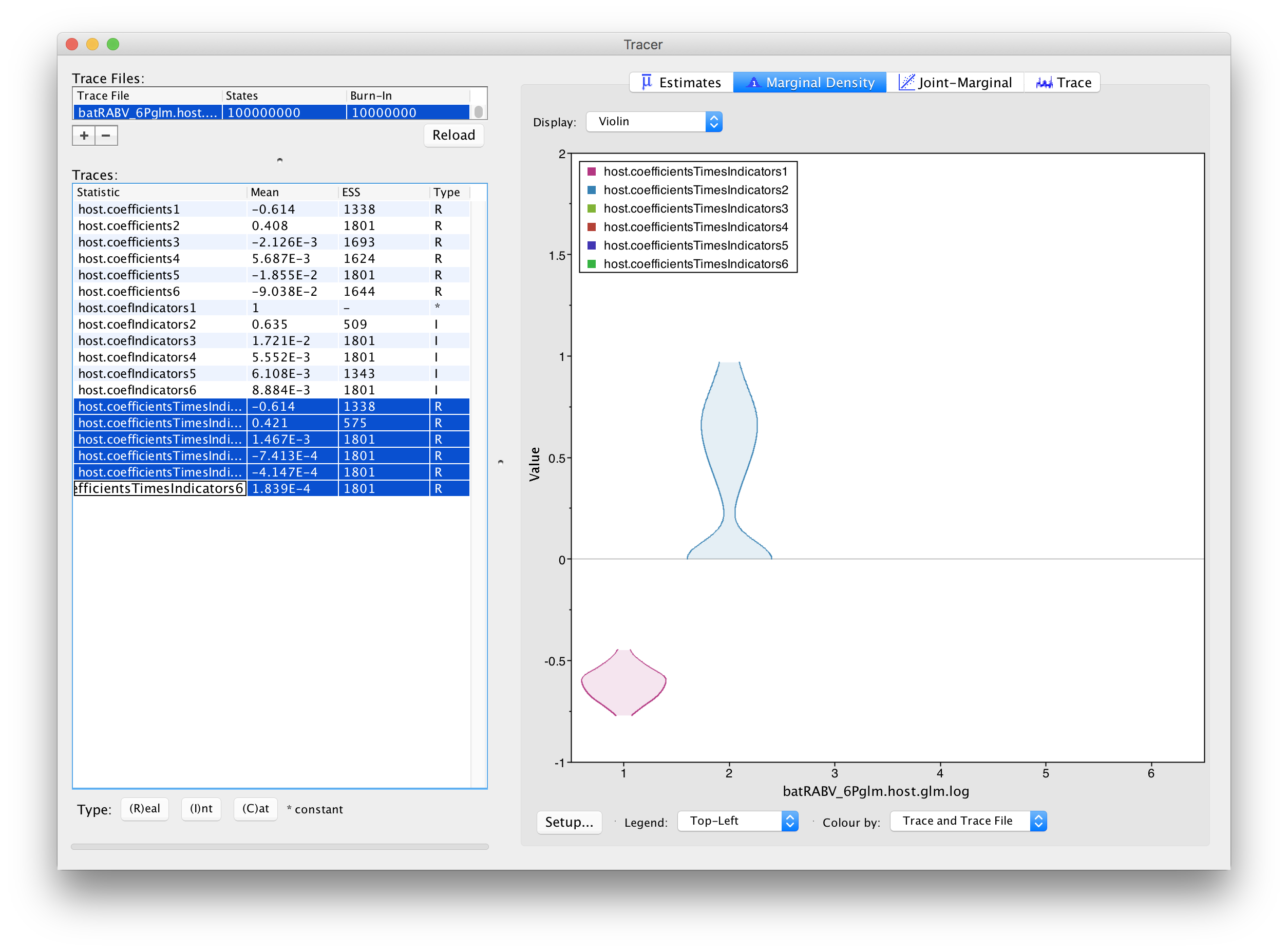
For host genetic distance (‘host.coefficientsTimesIndicators1’), the posterior density for this statistic is the same as for the actual coefficient (‘host.coefIndicators1’) because the associated indicator is always 1 for this predictor. The negative coefficient provides evidence for a higher intensity of host transitioning between more closely related hosts species. The posterior distribution for the statistic for range overlap (‘host.coefficientsTimesIndicators2’) shows a considerable density for positive values but also a non-negligible density at 0, as expected for its inclusion probability. So, although this predictor does not yield maximum support as the host genetic distances, it does suggest more intense transitioning between hosts with overlapping ranges.
Assessing the impact of sample sizes
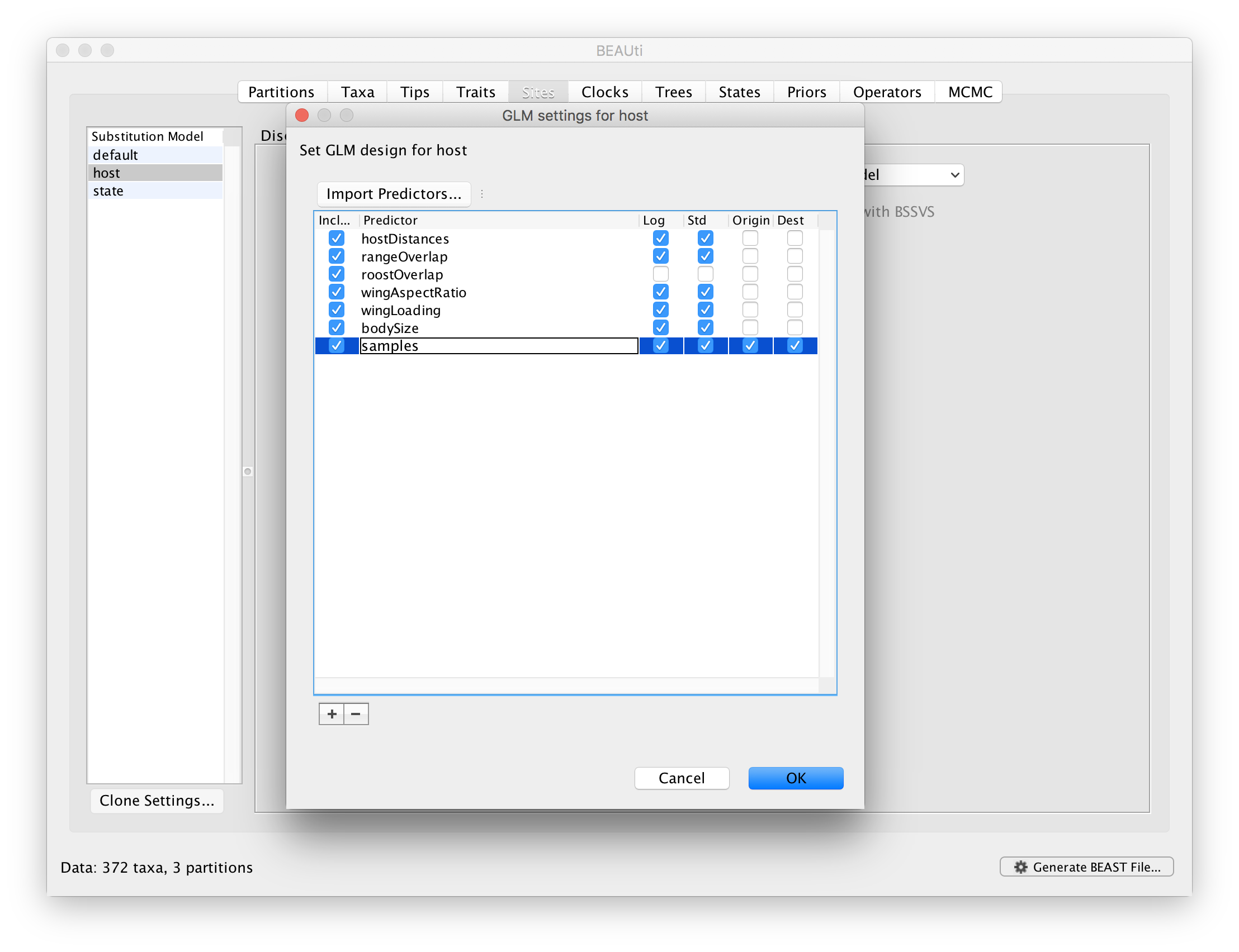
Sample sizes may have a strong impact on rate estimates in discrete ancestral reconstructions, and hence also on the GLM-parameters that parameterise these rates. In order to assess to what extent predictor inclusion is sensitive to sample sizes, we can explicitly include sample size as a predictor. However, sample size is a measure associated with a single discrete state and not measure between a pair of states. Therefore, we will include sample sizes both as an ‘donor’ and ‘recipient’ host measure. So for each pair of bat hosts, we will consider that sample size for both the donor and recipient in this pair can predict the intensity of host transitioning. The idea here is not to demonstrate the predictive power of sample sizes, but to assess whether the inclusion probabilities of the other predictors are sensitive to the inclusion/exclusion of sample sizes. To set up a GLM model including these sample saize predictors, go back to the GLM design window and import sampleSize.tsv as a predictor. Note that by default, both ‘Origin’ and ‘Destination’ will be selected:
References
- Streicker, D. G., A. S. Turmelle, M. J. Vonhof, I. V. Kuzmin, G. F. McCracken, and C. E. Rupprecht. 2010. Host phylogeny constrains cross-species emergence and establishment of rabies virus in bats. Science 329:676-679.
- Faria, N. R., M. A. Suchard, A. Rambaut, D. G. Streicker, and P. Lemey. 2013. Simultaneously reconstructing viral cross-species transmission history and identifying the underlying constraints. Philosophical transactions of the Royal Society of London. Series B, Biological sciences 368:20120196.
- Ferreira, M. A. R. and M. A. Suchard. 2008. Bayesian analysis of elapsed times in continuous-time Markov chains. Can J Statistics, 36: 355–368. doi: 10.1002/cjs.5550360302
- Lemey, P., A. Rambaut, A. J. Drummond, and M. A. Suchard. 2009. Bayesian phylogeography finds its roots. PLoS computational biology 5:e1000520.
- Lemey, P., A. Rambaut, T. Bedford, N. Faria, F. Bielejec, G. Baele, C. A. Russell, D. J. Smith, O. G. Pybus, D. Brockmann, and M. A. Suchard. 2014. Unifying Viral Genetics and Human Transportation Data to Predict the Global Transmission Dynamics of Human Influenza H3N2. PLoS pathogens 10:e1003932.
- Bloomquist, E. W., P. Lemey, and M. A. Suchard. 2010. Three roads diverged? Routes to phylogeographic inference. Trends Ecol Evol 25:626-632.## Help and documentation.
- Nahata KD, Bielejec F, Monetta J, Dellicour S, Rambaut A, Suchard MA, Baele G, Lemey P.. 2022. SPREAD 4: online visualisation of pathogen phylogeographic reconstructions. Virus Evol., 26;8(2):veac088. doi: 10.1093/ve/veac088. eCollection 2022.
Help and documentation
The BEAST website: http://beast.community
Tutorials: http://beast.community/tutorials
Frequently asked questions: http://beast.community/faq