Model selection and testing
Evaluating rate variation (using model selection)
To investigate lineage-specific rate heterogeneity in this data set and its impact on divergence date estimates, a log and trees file is available for an analysis using an uncorrelated lognormal relaxed clock.
Import this log file in Tracer in addition to the strict clock log file. Investigate the posterior density for the lognormal standard deviation; if this density excludes zero (= no rate variation), it would suggest that the strict clock model can be rejected in favor of the relaxed clock model.
A more formal test can be performed using a marginal likelihood estimator (MLE, Suchard et al., 2001, MBE 18: 1001-1013), which employs a mixture of model prior and posterior samples (Newton and Raftery 1994). The ratio of marginal likelihoods defines a Bayes factor, which measures the relative fit for two different models given the data at hand. Accurate estimation of the marginal likelihood is however not possible using Tracer, which has been shown on many occasions (Baele et al., 2012, 2013, 2016).
The harmonic mean estimator (HME) unfortunately remains a frequently used method to obtain marginal likelihood estimates, in large part because it’s so easily computed but it is more and more being disregarded as a reliable marginal likelihood estimator. To compare demographic and molecular clock models, both HME and sHME have been shown to be unreliable (Baele et al., 2012, 2013, 2016). More accurate/reliable MLE estimates can be obtained using computationally more demanding approaches, such as:
- Path sampling (PS)
- Proposed in the statistics literature over 2 decades ago (sometimes also referred to as ‘thermodynamic integration’), this approach has been introduced in phylogenetics in 2006 (Lartillot and Philippe 2006). Rather than only using samples from the posterior distribution, samples are required from a series of power posteriors between posterior and prior. As the power posterior gets closer to the prior, there is less and less data available for the posterior, which may lead to improper results when improper priors have been specified. The use of proper priors is hence of primary importance for PS (Baele et al., 2013, MBE, doi:10.1093/molbev/mss243).
- Stepping-stone sampling (SS)
- Following essentially the same approach as PS and using the same collection of samples from a series of power posteriors, stepping-stone sampling (SS) yields faster-converging results compared to PS. As was the case for PS, the use of proper priors is critical for SS.
- Generalised stepping-stone sampling (GSS)
- GSS combines the advantages of PS/SS — that they yield reliable estimates of the (log) marginal likelihood — with what has been a key attraction of the HME/AICM approach, i.e. that these approaches make use of the samples collected during the exploration of the posterior. GSS makes use of working distributions to shorten the path of the PS/SS integration and as such constructs a path between posterior and a product of working distributions, thereby avoiding exploration of the priors and the numerical issues associated with this (Baele et al., 2016, Syst. Biol., doi:10.1093/sysbio/syv083).
The aforementioned PS, SS and GSS approaches have been implemented in BEAST (Baele at al., 2012, 2016). Typically, PS/SS or GSS model selection is performed after doing a standard MCMC analysis and collecting samples from a series of power posteriors can then start where the MCMC analysis has stopped (i.e. you should have run the MCMC analysis long enough so that it converged towards the posterior), thereby eliminating the need for PS, SS and GSS to first converge towards the posterior.
As discussed earlier in the tutorial and in the theory on Bayesian model selection, obtaining reliable model comparison results requires the use of proper priors for all parameters being estimated. When performing model comparison, improper priors will lead to improper Bayes Factors. Further, for the PS/SS procedure, we need to sample from the prior at the end of the series of the power posteriors, which will be problematic without proper priors and lead to numerical instabilities (Baele at al., 2013, MBE, doi:10.1093/molbev/mss243).
Setting up a PS/SS analysis
To set up the analysis follow all the BEAUti steps in the Estimating rates and dates from time-stamped sequences tutorial up until the point of setting the MCMC panel options.
Specify a chain length of 1,000,000 and log parameters every 1,000 steps.
To set up the PS/SS analyses, in the MCMC panel select Marginal likelihood estimation (MLE): `path sampling / stepping-stone sampling’ as the technique we will use to perform marginal likelihood estimation:
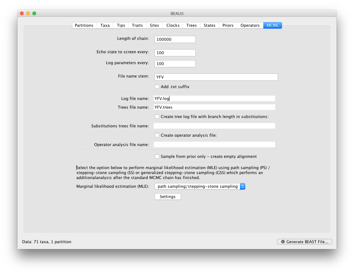
Click on Settings to specify the PS/SS settings.
Because of time constraints, we will collect samples from 11 power posteriors (i.e. 10 path steps between 1.0 and 0.0) so set Number of path steps: to 10. The length of the chain for the power posteriors can differ from the length of the standard MCMC chain, but we keep it here set to 100,000 as well.
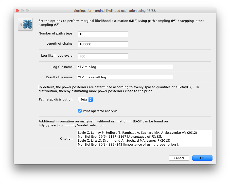
The powers for the different power posteriors are defined using evenly spaced quantiles of a Beta(\( \alpha \) ,1.0) distribution, with \( \alpha \) here equal to 0.30, as suggested in the stepping-stone sampling paper (Xie et al. 2011) since this approach is shown to outperform a uniform spreading suggested in the path sampling paper (Lartillot and Philippe 2006).
Note that there is an additional option available in the MLE panel: Print operator analysis.
When selected, this option will print an operator analysis for each power posterior to the screen, which can then be used to spot potential problems with the operators’ performance across the path from posterior to prior.
This option is useful when employing highly complex models and when having obtained improbable results.
Having set the PS/SS settings and proper priors, we can write to xml and run the analysis in BEAST. Use the same settings for the strict clock and the uncorrelated relaxed clock and run the analyses.
Important: in order to obtain reliable estimates for the marginal likelihoods using PS/SS, we need to rerun these analyses using much more demanding computational settings. For example, by setting the number of path steps to 50 and the length of the MCMC chain for each power posterior to 500,000 (the logging frequency could also be increased). The length of the initial standard MCMC chain should also be increased to ensure convergence towards the posterior before the PS/SS calculations are initiated. An initial chain length of 5,000,000 iterations should be sufficient here. Note that using these settings, the marginal likelihood estimation will take approximately the time it takes to complete a standard MCMC run of 25,000,000 generations for this data (+ 5,000,000 iterations for the initial chain). Due to time constraints, we won’t run this full-length analysis now (although more demanding computational settings can be attempted during the free computer time or left running over night).
Note: in early implementations of PS/SS/GSS in BEAST, the estimated log marginal likelihood estimate wasn’t saved to disk. Technically, simple XML files can be used when the actual MLE was lost but the log files are still available (which is a better alternative than rerunning the whole analysis). However, the latest release of BEAST saves the final result to a specified file name, so that this result is easily accessible, even when your terminal has been closed or your standard output is no longer available.
For the full-length strict clock analysis, we arrive at -5676.04 and -5676.10 for the log marginal likelihoods using PS and SS respectively. For the uncorrelated relaxed clock analysis, we get -5656.8 and -5658.14 for the same estimators.
Setting up a GSS analysis
To set up the GSS analyses, we can return to the MCMC panel in BEAUti and select ‘generalized stepping-stone sampling’ as the technique we will use to perform ‘Marginal likelihood estimation (MLE)’ in the MCMC panel.
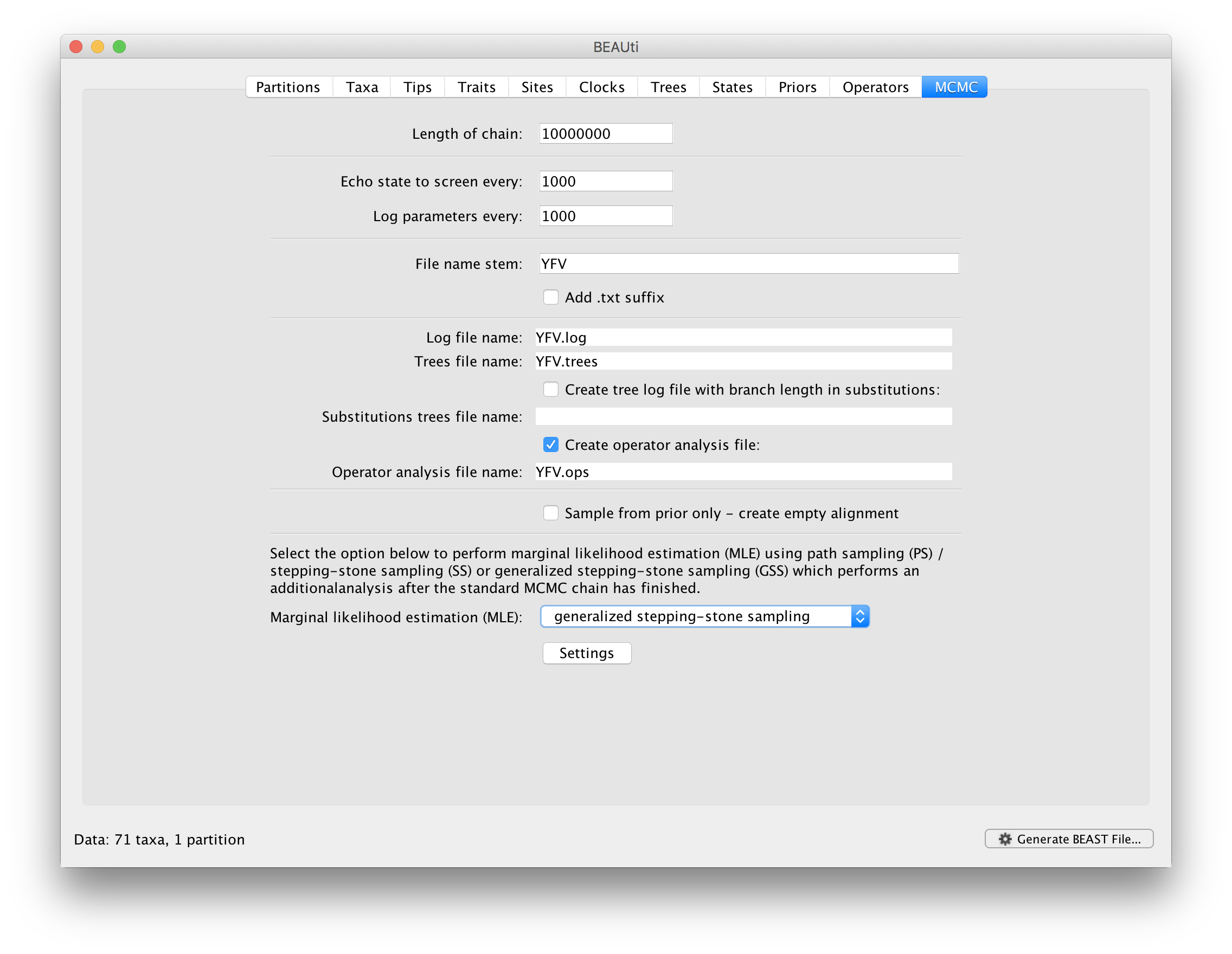
Click on ‘settings’ to specify the GSS settings. Because of time constraints, we will keep the length of the standard MCMC chain set to 1,000,000 and we will collect samples from 11 power posteriors (i.e. 10 path steps between 1.0 and 0.0). The length of the chain for the power posteriors can differ from the length of the standard MCMC chain, but we set it here to 100,000 as well. We again define the powers for the different power posteriors using evenly spaced quantiles of a Beta(0.3,1.0) distribution, since this has been shown to outperform a uniform spreading for generalised stepping-stone sampling (Baele et al., 2016).
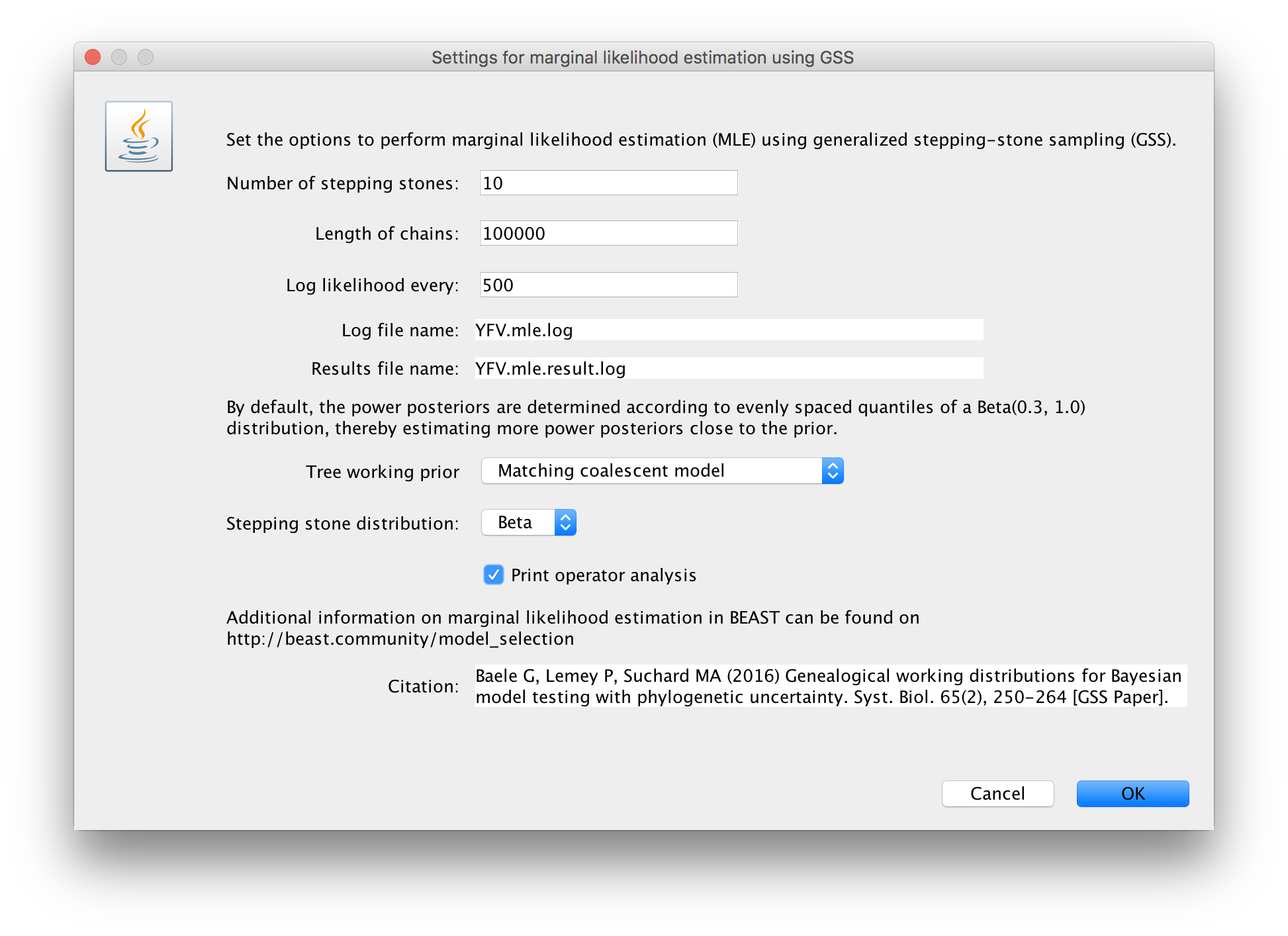
The working priors/distribution for the models’ parameters are automatically generated depending on their domain, but we need to make a choice when it comes to selecting a working prior for the tree topology. For parametric coalescent models, such as the constant population size model, the fastest approach is to use a ‘matching coalescent model’; whereas for non- parametric coalescent models, such as the Bayesian Skygrid model, the general-purpose ‘product of exponential distributions’ is the only appropriate option. Additionally, for speciation models (typically when using contemporaneous/isochronous sequences), the ‘matching speciation model’ is the only appropriate option.
The number of power posteriors needed as well as the chain length per power posterior are important settings to achieve a reliable estimate of the (log) marginal likelihood. However, these settings can depend on the data set being analysed and hence different PS/SS/GSS analyses (with differing computational settings) are required when performing model comparison. It’s strongly advised to estimate the MLE using PS/SS/GSS with increasing computational settings, until these values no longer change significantly, to ensure convergence to the correct MLE.
As discussed earlier, the model fit estimators used in this tutorial are not limited to specific types of models that can be compared. So apart from comparing different clock models to one another, we can use the same approaches to compare different evolutionary substitution models to one another, or different demographic models, … For example, try to compare the model fit of the HKY model of nucleotide substitution we’ve been using so far to a GTR model of nucleotide substitution.
References
Baele G., Lemey P., Bedford T., Rambaut A., Suchard M.A., Alekseyenko A.V. (2012) Improving the accuracy of demographic and molecular clock model comparison while accommodating phylogenetic uncertainty. Mol. Biol. Evol. 29:2157-2167.
Baele G., Li W.L.S., Drummond A.J., Suchard M.A., Lemey P. (2013) Accurate model selection of relaxed molecular clocks in Bayesian phylogenetics. Mol. Biol. Evol. 30:239-243.
Baele, G., Lemey, P., Suchard, M. A. (2016) Genealogical working distributions for Bayesian model testing with phylogenetic uncertainty. Syst. Biol. 65(2), 250-264.
Lartillot N., Philippe H. (2006) Computing Bayes factors using thermodynamic integration. Syst. Biol. 55:195-207.
Newton M.A., Raftery A.E. (1994) Approximating Bayesian inference with the weighted likelihood bootstrap. J. R. Stat. Soc. B. 56:3-48.
Suchard M.A., Weiss R.E., Sinsheimer J.S. (2001) Bayesian selection of continuous-time Markov chain evolutionary models. Mol. Biol. Evol. 18:1001-1013.
Xie W., Lewis P.O., Fan Y., Kuo L., Chen M.H. (2011) Improving marginal likelihood estimation for Bayesian phylogenetic model selection. Syst. Biol. 60:150-160.
Help and documentation
The BEAST website: http://beast.community
Tutorials: http://beast.community/tutorials
Frequently asked questions: http://beast.community/faq